Page 31 - Circuit Analysis II with MATLAB Applications

Response of Parallel GLC Circuits with DC Excitation

y2=diff(y0,2) % Compute and display second derivative
y2 =
776*exp(-4*t)-11136*exp(-16*t)

y=y2/640+y1/32+y0/10 % Verify that (1.40) is satisfied
y =
0

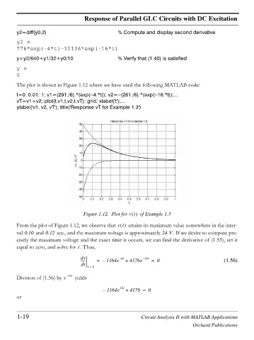
The plot is shown in Figure 1.12 where we have used the following MATLAB code:
t=0: 0.01: 1; v1=(291./6).*(exp( 4.*t)); v2= (261./6).*(exp( 16.*t));...
vT=v1+v2; plot(t,v1,t,v2,t,vT); grid; xlabel('t');...
ylabel('v1, v2, vT'); title('Response vT for Example 1.3')

Figure 1.12. Plot for vt of Example 1.3

From the plot of Figure 1.12, we observe that vt attains its maximum value somewhere in the inter-
val 0.10 and 0.12 sec., and the maximum voltage is approximately 24 V . If we desire to compute pre-
cisely the maximum voltage and the exact time it occurs, we can find the derivative of (1.55), set it
equal to zero, and solve for . Thus,
t

dv = – 1164e – 4t + 4176e – 16t = 0 (1.56)
------
dt
t = 0
Division of (1.56) by e – 16t yields

– 1164e 12t + 4176 = 0
or

1-19 Circuit Analysis II with MATLAB Applications
Orchard Publications