Page 35 - Circuit Analysis II with MATLAB Applications

Response of Parallel GLC Circuits with DC Excitation

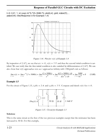
t=0: 0.01: 1; vt=exp( 8.*t).*(5+5080.*t); plot(t,vt); grid; xlabel('t');...
ylabel('vt'); title('Response vt for Example 1.4')

Figure 1.14. Plot for vt of Example 1.4

By inspection of (1.67), we see that at t = , 0 vt = 5V and thus the second initial condition is sat-
isfied. We can verify that the first initial condition is also satisfied by differentiation of (1.67). We can
t
also show that vt approaches zero as approaches infinity with L’Hôpital’s rule as follows:
5080t
5 +

---------------------------------------- =
------------ =
lim vt lim e = – 8t 5 + 5080t = lim ---------------------------- = lim d 5 + 5080t e dt lim 5080 0 (1.68)

t o f t o f t o f e 8t t o f de 8t e dt t o f 8e 8t
Example 1.5
For the circuit of Figure 1.15, i 0 = 2A and v 0 = 5V . Compute and sketch vt for t ! . 0
C
L
i R i L i C
`
vt
10u t A 50 : 10 H 1 640 F
e
0

Figure 1.15. Circuit for Example 1.5

Solution:

This is the same circuit as the that of the two previous examples except that the resistance has been
increased to 50 : . For this example,

1-23 Circuit Analysis II with MATLAB Applications
Orchard Publications