Page 38 - Circuit Analysis II with MATLAB Applications

Chapter 1 Second Order Circuits

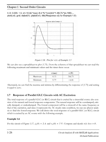
t=0: 0.005: 1.5; vt=10.42.*exp( 6.4.*t).*cos(4.8.*t 89.73.*pi./180);...
plot(t,vt); grid; xlabel('t'); ylabel('vt'); title('Response v(t) for Example 1.5')

Figure 1.16. Plot for vt of Example 1.5
We can also use a spreadsheet to plot (1.75). From the columns of that spreadsheet we can read the
following maximum and minimum values and the times these occur.

t (sec) v (V)
Maximum 0.13 266.71
Minimum 0.79 4.05

Alternately, we can find the maxima and minima by differentiating the response of (1.75) and setting
it equal to zero.

1.7 Response of Parallel GLC Circuits with AC Excitation

The total response of a parallel GLC (or RLC) circuit that is excited by a sinusoidal source also con-
sists of the natural and forced response components. The natural response will be overdamped, criti-
cally damped, or underdamped. The forced component will be a sinusoid of the same frequency as
that of the excitation, and since it represents the AC steady-state condition, we can use phasor analy-
sis to find the forced response. We will derive the total response of a parallel GLC (or RLC) circuit
which is excited by an AC source with the following example.

Example 1.6

For the circuit of Figure 1.17, i 0 = 2A and v 0 = 5V . Compute and sketch vt for t ! 0 .
C
L

1-26 Circuit Analysis II with MATLAB Applications
Orchard Publications