Page 26 - Circuit Analysis II with MATLAB Applications

Chapter 1 Second Order Circuits

Simultaneous solution of (1.34) and (1.38) yields k = – 38 and k = 42 . Then, by substitution into
2
1
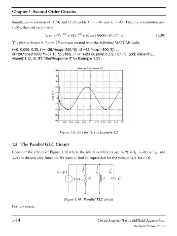
(1.31), the total response is
it = – 38e – 200t + 42e – 300t + 20cos 10000t 87.15 – o A (1.39)
The plot is shown in Figure 1.9 and was created with the following MATLAB code:

t=0: 0.005: 0.20; i1= 38.*(exp( 200.*t)); i2=42.*(exp( 300.*t));...
i3=20.*cos(10000.*t 87.15.*pi./180); iT=i1+i2+i3; plot(t,i1,t,i2,t,i3,t,iT); grid; xlabel('t');...
ylabel('i1, i2, i3, iT'); title('Response iT for Example 1.2')

Figure 1.9. Plot for it of Example 1.2

1.5 The Parallel GLC Circuit

Consider the circuit of Figure 1.10 where the initial conditions are i 0 = I 0 , v 0 = V 0 , and
C
L
u t is the unit step function. We want to find an expression for the voltage vt for t ! 0 .
0

i u t i G i L i C
0
S
vt G ` L C

Figure 1.10. Parallel RLC circuit

For this circuit

1-14 Circuit Analysis II with MATLAB Applications
Orchard Publications