Page 23 - Circuit Analysis II with MATLAB Applications

Response of Series RLC Circuits with AC Excitation

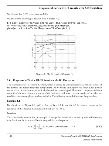
We observe that (1.29) is the same as (1.17).

We will use the following MATLAB code to sketch it .
t=0: 0.001: 0.03; vc1=22.*(exp( 300.*t)); vc2= 34.5.*(exp( 200.*t)); vc3=15;...
vcT=vc1+vc2+vc3; plot(t,vc1,t,vc2,t,vc3,t,vcT); grid; xlabel('t');...
ylabel('vc1, vc2, vc3, vcT'); title('Response vcT for Example 1.1')

Figure 1.7. Plot for v t of Example 1.1
C
1.4 Response of Series RLC Circuits with AC Excitation

The total response of a series RLC circuit, which is excited by a sinusoidal source, will also consist of
the natural and forced response components. As we found in the previous section, the natural
response can be overdamped, or critically damped, or underdamped. The forced component will be a
sinusoid of the same frequency as that of the excitation, and since it represents the AC steady-state
condition, we can use phasor analysis to find it. The following example illustrates the procedure.

Example 1.2

For the circuit of Figure 1.8, i 0 = 5A , v 0 = 2.5 V , and the 0.5 : resistor represents the
L
C
resistance of the inductor. Compute and sketch it for t ! . 0
Solution:

This circuit is the same as that of Example 1.1 except that the circuit is excited by a sinusoidal source;
therefore it can be represented by the integrodifferential equation

di 1 t
Ri + L----- + ---- ³ it + v 0 = 200cos 10000t t ! 0 (1.30)
d
dt C 0 C

1-11 Circuit Analysis II with MATLAB Applications
Orchard Publications