Page 103 - Classification Parameter Estimation & State Estimation An Engg Approach Using MATLAB

92 STATE ESTIMATION

b) 5 α = 0.95; σ =1
w
+1σ boundary
0

–1σ boundary
–5
0 50 100
a) c)
40 α = 1.02; σ =1
w
w(i ) 20
+1σ boundary
x(i + 1) 0
+ buffer x(i )
–20 –1σ boundary
α
–40
0 50 i 100
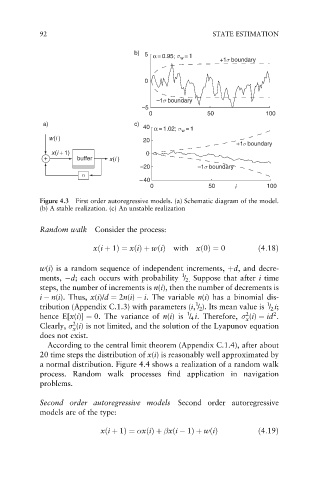
Figure 4.3 First order autoregressive models. (a) Schematic diagram of the model.
(b) A stable realization. (c) An unstable realization

Random walk Consider the process:

xði þ 1Þ¼ xðiÞþ wðiÞ with xð0Þ¼ 0 ð4:18Þ

w(i) is a random sequence of independent increments, þd, and decre-
1
ments, d; each occurs with probability / 2. Suppose that after i time
steps, the number of increments is n(i), then the number of decrements is
i n(i). Thus, x(i)/d ¼ 2n(i) i. The variable n(i) has a binomial dis-
1
1
tribution (Appendix C.1.3) with parameters (i, / 2 ). Its mean value is / 2 i;
1
2
2
hence E[x(i)] ¼ 0. The variance of n(i)is / 4 i. Therefore, (i) ¼ id .
x
2
Clearly, (i) is not limited, and the solution of the Lyapunov equation
x
does not exist.
According to the central limit theorem (Appendix C.1.4), after about
20 time steps the distribution of x(i) is reasonably well approximated by
a normal distribution. Figure 4.4 shows a realization of a random walk
process. Random walk processes find application in navigation
problems.
Second order autoregressive models Second order autoregressive
models are of the type:

xði þ 1Þ¼ xðiÞþ xði 1Þþ wðiÞ ð4:19Þ