Page 108 - Classification Parameter Estimation & State Estimation An Engg Approach Using MATLAB

CONTINUOUS STATE VARIABLES 97

The discrete Kalman filter
The concepts developed in the previous section are sufficient to trans-
form the general scheme presented in Section 4.1 into a practical solu-
tion. In order to develop the estimator, first the initial condition valid for
i ¼ 0 must be established. In the general case, this condition is defined in
terms of the probability density p(x(0)) for x(0). Assuming a normal
distribution for x(0) it suffices to specify only the expectation E[x(0)]
and the covariance matrix C x (0). Hence, the assumption is that these
parameters are available. If not, we can set E[x(0)] ¼ 0 and let C x (0)
approach to infinity, i.e. C x (0) !1I. Such a large covariance matrix
represents the lack of prior knowledge.
The next step is to establish the posterior density p(x(0)jz(0)) from
which the optimal estimate for x(0) follows. At this point, we enter the
loop of Figure 4.2. Hence, we calculate the density p(x(1)jz(0)) of the
next state, and process the measurement z(1) resulting in the updated
density p(x(1)jz(0), z(1)) ¼ p(x(1)jZ(1)). From that, the optimal estimate
for x(1) follows. This procedure has to be iterated for all the next time
cycles.
The representation of all the densities that are involved can be given
in terms of expectations and covariances. The reason is that any linear
combination of Gaussian random vectors yields a vector that is also
Gaussian. Therefore, both p(x(i þ 1)jZ(i)) and p((x(i)jZ(i)) are fully
represented by their expectations and covariances. In order to discrim-
inate between the two situations a new notation is needed. From
now on, the conditional expectation E[x(i)jZ(j)] will be denoted by
x(ijj). It is the expectation associated with the conditional density
p(x(i)jZ(j)). The covariance matrix associated with this density is
denoted by C(ijj).
The update, i.e. the determination of p((x(i)jZ(i)) given p(x(i)j
Z(i 1)), follows from Section 3.1.5 where it has been shown that the
unbiased linear MMSE estimate in the linear-Gaussian case equals the
MMSE estimate, and that this estimate is the conditional expectation.
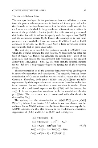
Application of (3.33) and (3.45) to (4.25) and (4.26) gives:

z ^ zðiÞ¼ HðiÞxðiji 1Þ
T
SðiÞ¼ HðiÞCðiji 1ÞH ðiÞþ C v ðiÞ
T 1
KðiÞ¼ Cðiji 1ÞH ðiÞS ðiÞ ð4:27Þ
z
ð
xðii j Þ¼ xðiji 1Þþ KðiÞ zðiÞ ^ zðiÞÞ
T
Cðii j Þ¼ Cðiji 1Þ KðiÞSðiÞK ðiÞ