
Page 104 - Classification Parameter Estimation & State Estimation An Engg Approach Using MATLAB
P. 104
CONTINUOUS STATE VARIABLES 93
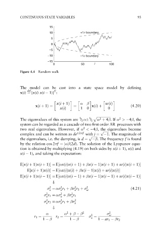
15
10 +1σ boundary
5
0
–5
–10 –1σ boundary
–15
0 50 i 100
Figure 4.4 Random walk
The model can be cast into a state space model by defining
def T
x(i) ¼ [x(i) x(i 1)] :
xði þ 1Þ wðiÞ
xði þ 1Þ¼ ¼ xðiÞþ ð4:20Þ
xðiÞ 1 0 0
1 1 p ffiffiffiffiffiffiffiffiffiffiffiffiffiffiffiffiffi 2
2
The eigenvalues of this system are / 2 / 2 þ 4 .If > 4 , the
system can be regarded as a cascade of two first order AR processes with
2
two real eigenvalues. However, if < 4 , the eigenvalues become
p ffiffiffiffiffiffiffi
complex and can be written as de 2 jf with j ¼ 1. The magnitude of
p ffiffiffiffiffiffiffi
the eigenvalues, i.e. the damping, is d ¼ . The frequency f is found
by the relation cos 2 f ¼ jj/(2d). The solution of the Lyapunov equa-
tion is obtained by multiplying (4.19) on both sides by x(i þ 1), x(i) and
x(i 1), and taking the expectation:
E½xði þ 1Þxði þ 1Þ ¼ E½ xðiÞxði þ 1Þþ xði 1Þxði þ 1Þþ wðiÞxði þ 1Þ
E½xði þ 1ÞxðiÞ ¼ E½ xðiÞxðiÞþ xði 1ÞxðiÞþ wðiÞxðiÞ
E½xði þ 1Þxði 1Þ ¼ E½ xðiÞxði 1Þþ xði 1Þxði 1Þþ wðiÞxði 1Þ
+
2
2
2
¼ r 1 þ r 2 þ 2 w ð4:21Þ
x
x
x
2 2 2
r 1 ¼ þ r 1
x x x
2
2
r 2 ¼ r 1 þ 2 x
x
x
+
2
þ 2 2 2 w
r 1 ¼ r 2 ¼ ¼
x
1 1 1 ar 1 r 2