Page 106 - Classification Parameter Estimation & State Estimation An Engg Approach Using MATLAB

CONTINUOUS STATE VARIABLES 95

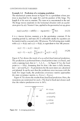
Example 4.2 Prediction of a swinging pendulum
The mechanical system shown in Figure 4.6 is a pendulum whose pos-
ition is described by the angle (t) and the position of the hinge. The
length R of the arm is constant. The mass m is concentrated at the end.
The hinge moves randomly in the horizontal direction with an acceler-
ation given by a(t). Newton’s law, applied to the geometrical set up, gives:

mk
€
_

maðtÞ cos ðtÞþ mR ðtÞ¼ mg sin ðtÞ ðtÞ ð4:23Þ
R
k is a viscous friction constant; g is the gravitation constant. If the
sampling period ,andmax (jyj) is sufficiently small, the equation can
be transformed to a second order AR process. The following state model,
_

with x 1 (i) ¼ (i )and x 2 (i) ¼ (i ), is equivalent to that AR process:
x 1 ði þ 1Þ¼ x 1 ðiÞþ x 2 ðiÞ
k ð4:24Þ
x 2 ði þ 1Þ¼ x 2 ðiÞ gx 1 ðiÞþ x 2 ðiÞþ aðiÞ
R R
Figure 4.7(a) shows the result of a so-called fixed interval prediction.
The prediction is performed from a fixed point in time (i is fixed), and
with a running lead, that is ‘ ¼ 1, 2, 3, .. . . In Figure 4.7(a), the fixed
point is i 10(s). Assuming that for that i the state is fully known,
^ x x(i) ¼ x(i) and C e (i) ¼ 0, predictions for the next states are calculated
and plotted. It can be seen that the prediction error increases with the
lead. For larger leads, the prediction covariance matrix approaches
the state covariance matrix, i.e. C e (1) ¼ C x (1).
Figure 4.7(b) shows the results from fixed lead prediction. Here, the
recursions are reinitiated for each i. The lead is fixed and chosen such
that the relative prediction error is 36%.

R = 1.5 (m)
a (t)
2
g = 9.8 (m/s )
R θ(t) k = 0.2 (m /s)
2
∆ = 0.01(s)
2
σ = 1 (m/s )
a
m
Figure 4.6 A swinging pendulum