Page 143 - Classification Parameter Estimation & State Estimation An Engg Approach Using MATLAB
P. 143
132                                            STATE ESTIMATION

            for p(x(i)jZ(i)), the representation of p(x(i þ 1)jZ(i)) is found by
            generating one new sample x   (k)  for each sample x (k)    using
                                                                 selected
            p(x(i þ 1)jx (k)  ) as the density to draw from. The algorithm is as
                      selected
            follows:
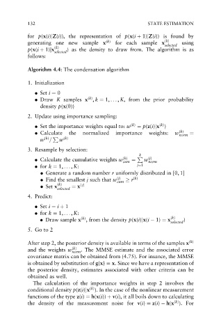
            Algorithm 4.4: The condensation algorithm


            1. Initialization
               . Set i ¼ 0
                                   (k)
               . Draw K samples x , k ¼ 1, ... , K, from the prior probability
                 density p(x(0))

            2. Update using importance sampling:
                                                               (k)
               . Set the importance weights equal to: w (k)  ¼ p(z(i)jx )
               . Calculate  the  normalized   importance   weights:  w (k)  ¼
                                                                       norm
                  (k)
                 w =  P  w (k)
            3. Resample by selection:
                                                       k
               . Calculate the cumulative weights w (k)  ¼  P  w (j)
                                                           norm
                                                 cum
               . for k ¼ 1, ... , K:                  j¼1
                 . Generate a random number r uniformly distributed in [0, 1]
                 . Find the smallest j such that w (j)    r (k)
                                               cum
                 . Set x (k)  ¼ x ( j)
                       selected
            4. Predict:

               . Set i ¼ i þ 1
               . for k ¼ 1, ... , K:
                                 (k)
                 . Draw sample x , from the density p(x(i)jx(i   1) ¼ x (k)  )
                                                                   selected
            5. Go to 2

            After step 2, the posterior density is available in terms of the samples x (k)
            and the weights w (k)  . The MMSE estimate and the associated error
                             norm
            covariance matrix can be obtained from (4.75). For insance, the MMSE
            is obtained by substitution of g(x) ¼ x. Since we have a representation of
            the posterior density, estimates associated with other criteria can be
            obtained as well.
              The calculation of the importance weights in step 2 involves the
                                    (k)
            conditional density p(z(i)jx ). In the case of the nonlinear measurement
            functions of the type z(i) ¼ h(x(i)) þ v(i), it all boils down to calculating
                                                                     (k)
            the density of the measurement noise for v(i) ¼ z(i)   h(x ). For

