Page 186 - Classification Parameter Estimation & State Estimation An Engg Approach Using MATLAB

NONPARAMETRIC LEARNING 175

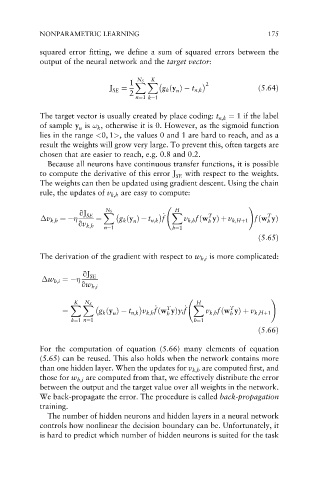
squared error fitting, we define a sum of squared errors between the
output of the neural network and the target vector:

K
1 X X 2
N S
J SE ¼ g k ðy Þ t n;k ð5:64Þ
n
2
n¼1 k¼1
The target vector is usually created by place coding: t n,k ¼ 1 if the label
of sample y is ! k , otherwise it is 0. However, as the sigmoid function
n
lies in the range <0, 1>, the values 0 and 1 are hard to reach, and as a
result the weights will grow very large. To prevent this, often targets are
chosen that are easier to reach, e.g. 0.8 and 0.2.
Because all neurons have continuous transfer functions, it is possible
to compute the derivative of this error J SE with respect to the weights.
The weights can then be updated using gradient descent. Using the chain
rule, the updates of v k,h are easy to compute:

!
H
qJ X X
N S
T
T
v k;h ¼ SE ¼ g k ðy Þ t n;k f f _ v k;h fðw yÞþ v k;Hþ1 fðw yÞ
h
h
n
qv k;h
n¼1 h¼1
ð5:65Þ
The derivation of the gradient with respect to w h,i is more complicated:
qJ
w h;i ¼ SE
qw h;i
K N S H !
X X
_ T _ X T
f
¼ g k ðy Þ t n;k v k;h fðw yÞy i f f v k;h fðw yÞþ v k;Hþ1
h
h
n
k¼1 n¼1 h¼1
ð5:66Þ
For the computation of equation (5.66) many elements of equation
(5.65) can be reused. This also holds when the network contains more
than one hidden layer. When the updates for v k,h are computed first, and
those for w h,i are computed from that, we effectively distribute the error
between the output and the target value over all weights in the network.
We back-propagate the error. The procedure is called back-propagation
training.
The number of hidden neurons and hidden layers in a neural network
controls how nonlinear the decision boundary can be. Unfortunately, it
is hard to predict which number of hidden neurons is suited for the task