Page 190 - Classification Parameter Estimation & State Estimation An Engg Approach Using MATLAB

EMPIRICAL EVALUATION 179

capability and the storage capability are subjected to constraints. At the
same time, the application may limit the computational time needed for
the classification. Often, a trade-off must be found between computa-
tional complexity and performance. In order to do so, we have to assess
the number of operations per classification and the storage require-
ments. These aspects scale with the number of elements N in the
measurement vector, the number of classes K, and for some classifiers
the size N S of the training set. For instance, the number of operations of
2
a quadratic machine is of the order of KN , and so is its memory
requirement. For binary measurements, the storage requirement is of
N
the order of K2 (which becomes prohibitive even for moderate N).
Often, the acquisition of labelled samples is laborious and costly.
Therefore, it is tempting to use the training set also for evaluation
purposes. However, the strategy of ‘testing from training data’ disguises
the phenomenon of overfitting. The estimated error rate is likely to be
strongly overoptimistic. To prevent this, the validation set should be
independent of the training set.
A straightforward way to accomplish this is the so-called holdout
method. The available samples are randomly partitioned into a training
set and a validation set. Because the validation set is used to estimate
only one parameter, i.e. the error rate, and the training set is used to
tune all other parameters of the classifier (which may be quite numer-
ous), the training set must be larger than the validation set. As a rule of
thumb, the validation set contains about 20% of the data, and the
training set the remaining 80%.
Suppose that a validation set consisting of, say, N Test labelled samples
is available. Application of the ‘classifier-under-test’ to this validation
set results in n error misclassified samples. If the true error rate of the
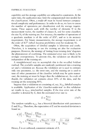
classifier is denoted by E, then the estimated error rate is:
^ n error
E E ¼ ð5:67Þ
N Test
The random variable n error has a binomial distribution with parameters
^
E
E and N Test . Therefore, the expectation of E and its standard deviation is
found as:
hi E½n error Š
^ EN Test
E
E E ¼ ¼ ¼ E
N Test N Test
ð5:68Þ
s ffiffiffiffiffiffiffiffiffiffiffiffiffiffiffiffiffiffiffi
p ffiffiffiffiffiffiffiffiffiffiffiffiffiffiffiffiffiffiffiffiffi p ffiffiffiffiffiffiffiffiffiffiffiffiffiffiffiffiffiffiffiffiffiffiffiffiffiffiffiffiffiffi
Var½n error Š N Test ð1 EÞE ð1 EÞE
¼ ¼ ¼
^ E
E
N Test N Test N Test
^
Hence, E is an unbiased, consistent estimate of E.
E