Page 86 - Classification Parameter Estimation & State Estimation An Engg Approach Using MATLAB
P. 86
DATA FITTING                                                  75

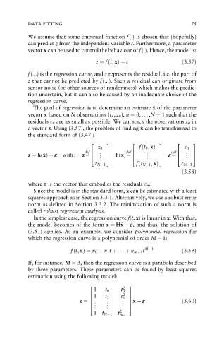
            We assume that some empirical function f(:) is chosen that (hopefully)
            can predict z from the independent variable t. Furthermore, a parameter
            vector x can be used to control the behaviour of f(:). Hence, the model is:

                                      z ¼ fðt; xÞþ "                   ð3:57Þ

            f(:,:) is the regression curve, and " represents the residual, i.e. the part of
            z that cannot be predicted by f(:,:). Such a residual can originate from
            sensor noise (or other sources of randomness) which makes the predic-
            tion uncertain, but it can also be caused by an inadequate choice of the
            regression curve.
              The goal of regression is to determine an estimate ^ x of the parameter
                                                            x
            vector x based on N observations (t n , z n ), n ¼ 0, .. . ,N   1 such that the
            residuals " n are as small as possible. We can stack the observations z n in
                                                       x
            a vector z. Using (3.57), the problem of finding ^ x can be transformed to
            the standard form of (3.47):
                                    2     3         2         3      2     3
                                       z 0            fðt 0 ; xÞ        " 0
            z ¼ hð^ xÞþ e  with:  z¼4  . . .  7  def6    . . .  7  e ¼4  . . .  7
                 x
                                  def6
                                                                   def6
                                          5 hðxÞ¼4
                                                              5
                                                                           5
                                     z N 1           fðt N 1 ; xÞ      " N 1
                                                                       ð3:58Þ
            where e is the vector that embodies the residuals " n .
              Since the model is in the standard form, x can be estimated with a least
            squares approach as in Section 3.3.1. Alternatively, we use a robust error
            norm as defined in Section 3.3.2. The minimization of such a norm is
            called robust regression analysis.
              In the simplest case, the regression curve f(t, x) is linear in x. With that,
                                               x
            the model becomes of the form z ¼ H^ x þ e, and thus, the solution of
            (3.51) applies. As an example, we consider polynomial regression for
            which the regression curve is a polynomial of order M   1:

                            fðt; xÞ¼ x 0 þ x 1 t þ      þ x M 1 t M 1  ð3:59Þ

            If, for instance, M ¼ 3, then the regression curve is a parabola described
            by three parameters. These parameters can be found by least squares
            estimation using the following model:


                                     1   t 0   t 0
                                   2            2  3
                                     1         t
                                   6     t 1    2 7
                                                    x
                                   6            . 7^ x þ e
                                     .    .                            ð3:60Þ
                                                1 7
                                z ¼ 6  .  .
                                   4  .   .     . . 5
                                     1 t N 1  t 2
                                               N 1

