Page 89 - Classification Parameter Estimation & State Estimation An Engg Approach Using MATLAB

78 PARAMETER ESTIMATION

fitting
Bayes estimation
techniques

quadratic uniform robust
cost function cost function error norm

MMSE MAP robust
estimation estimation sum of estimation
= squared
minimum variance difference
estimation prior knowledge norm function
not available fitting
linearity
constraints ML robust
estimation regression
analysis
unbiased linear LS
MMSE Gaussian estimation
estimation white noise

linear Gaussian
sensors densities linear function
+ sensors fitting
Gaussian
additive white noise +
noise linear sensors
Kalman pseudo regression
form inverse analysis

MMSE = minimum mean square error
MAP = maximum a posteriori
ML = maximum likelihood
LS = least squares
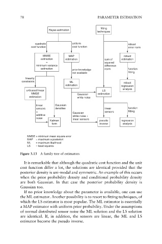
Figure 3.13 A family tree of estimators

It is remarkable that although the quadratic cost function and the unit
cost function differ a lot, the solutions are identical provided that the
posterior density is uni-modal and symmetric. An example of this occurs
when the prior probability density and conditional probability density
are both Gaussian. In that case the posterior probability density is
Gaussian too.
If no prior knowledge about the parameter is available, one can use
the ML estimator. Another possibility is to resort to fitting techniques, of
which the LS estimator is most popular. The ML estimator is essentially
a MAP estimator with uniform prior probability. Under the assumptions
of normal distributed sensor noise the ML solution and the LS solution
are identical. If, in addition, the sensors are linear, the ML and LS
estimator become the pseudo inverse.