Page 87 - Classification Parameter Estimation & State Estimation An Engg Approach Using MATLAB

76 PARAMETER ESTIMATION

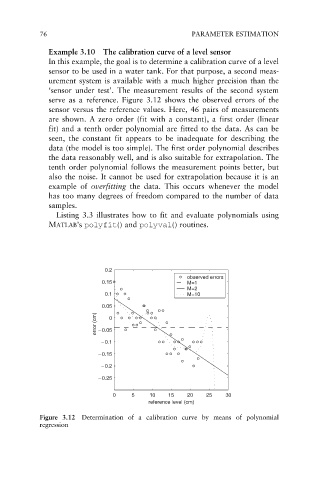
Example 3.10 The calibration curve of a level sensor
In this example, the goal is to determine a calibration curve of a level
sensor to be used in a water tank. For that purpose, a second meas-
urement system is available with a much higher precision than the
‘sensor under test’. The measurement results of the second system
serve as a reference. Figure 3.12 shows the observed errors of the
sensor versus the reference values. Here, 46 pairs of measurements
are shown. A zero order (fit with a constant), a first order (linear
fit) and a tenth order polynomial are fitted to the data. As can be
seen, the constant fit appears to be inadequate for describing the
data (the model is too simple). The first order polynomial describes
the data reasonably well, and is also suitable for extrapolation. The
tenth order polynomial follows the measurement points better, but
also the noise. It cannot be used for extrapolation because it is an
example of overfitting the data. This occurs whenever the model
has too many degrees of freedom compared to the number of data
samples.
Listing 3.3 illustrates how to fit and evaluate polynomials using
MATLAB’s polyfit() and polyval() routines.

0.2
observed errors
0.15 M=1
M=2
0.1 M=10
0.05
error (cm) – 0.05 0

– 0.1
– 0.15
– 0.2

– 0.25
0 5 10 15 20 25 30
reference level (cm)
Figure 3.12 Determination of a calibration curve by means of polynomial
regression