Page 242 - Classification Parameter Estimation & State Estimation An Engg Approach Using MATLAB

CLUSTERING 231

(a) (b)
2 6
1.8
5
1.6
1.4
4
1.2
distance 1 distance 3
0.8
2
0.6
0.4
1
0.2
0 0
1 5 2 4 3 6 1 5 2 4 3 6
object object
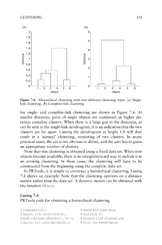
Figure 7.6 Hierarchical clustering with two different clustering types. (a) Single-
link clustering. (b) Complete-link clustering
for single- and complete-link clustering are shown in Figure 7.6. At
smaller distances, pairs of single objects are combined, at higher dis-
tances complete clusters. When there is a large gap in the distances, as
can be seen in the single-link dendrogram, it is an indication that the two
clusters are far apart. Cutting the dendrogram at height 1.0 will then
result in a ‘natural’ clustering, consisting of two clusters. In many
practical cases, the cut is not obvious to define, and the user has to guess
an appropriate number of clusters.
Note that this clustering is obtained using a fixed data set. When new
objects become available, there is no straightforward way to include it in
an existing clustering. In these cases, the clustering will have to be
constructed from the beginning using the complete data set.
In PRTools, it is simple to construct a hierarchical clustering; Listing
7.4 shows an example. Note that the clustering operates on a distance
matrix rather than the data set. A distance matrix can be obtained with
the function distm.

Listing 7.4
PRTools code for obtaining a hierarchical clustering.

z ¼ gendats(5); % Generate some data
figure; clf; scatterd(z); % and plot it
dendr ¼ hclust(distm(z),‘s’); % Single link clustering
figure; clf; plotdg(dendr); % Plot the dendrogram