Page 40 - Classification Parameter Estimation & State Estimation An Engg Approach Using MATLAB

BAYESIAN CLASSIFICATION 29

where:

T
w k ¼ 2ln Pð! k Þ m C m
1
k k
ð2:26Þ
w k ¼ 2C m k
1
A decision function which has the form of (2.25) is linear. The corre-
sponding classifier is called a linear classifier. The equations of the
T
decision boundaries are w i w j þ z (w i w j ) ¼ 0.
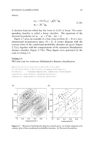
Figure 2.7 gives an example of a four-class problem (K ¼ 4) in a two-
dimensional measurement space (N ¼ 2). A scatter diagram with the
contour plots of the conditional probability densities are given (Figure
2.7(a)), together with the compartments of the minimum Mahalanobis
distance classifier (Figure 2.7(b)). These figures were generated by the
code in Listing 2.3.

Listing 2.3
PRTools code for minimum Mahalanobis distance classification

mus ¼ [0.2 0.3; 0.35 0.75; 0.65 0.55; 0.8 0.25];
C ¼ [0.018 0.007; 0.007 0.011]; z ¼ gauss(200,mus,C);
w ¼ ldc(z); % Normal densities, identical covariances
figure(1); scatterd(z); hold on; plotm(w);
figure(2); scatterd(z); hold on; plotc(w);

(a) (b)
1 1

0.8 0.8
measurement 2 0.6 measurement 2 0.6

0.4
0.4

0.2 0.2

0 0
0 0.2 0.4 0.6 0.8 1 0 0.2 0.4 0.6 0.8 1
measurement 1 measurement1

Figure 2.7 Minimum Mahalanobis distance classification. (a) Scatter diagram with
contour plot of the conditional probability densities. (b) Decision boundaries