Page 41 - Classification Parameter Estimation & State Estimation An Engg Approach Using MATLAB
P. 41

30                               DETECTION AND CLASSIFICATION

            Minimum distance classification
            A further simplification is possible when the measurement vector equals
            the class-dependent vector m corrupted by class-independent white
                                       k
                                            2
            noise with covariance matrix C ¼   I.
                                                                2
                                          (                      )
                                                         kz   m k
                                                              k
                ^ ! !ðzÞ¼ ! i  with i ¼ argmin  2ln Pð! k Þþ  2        ð2:27Þ
                                    k¼1;...;K
            The quantity k(z   m )k is the normal (Euclidean) distance between z
                               k
            and m . The classifier corresponding to (2.27) decides for the class whose
                 k
            expectation vector is nearest to the observed measurement vector (with a
                                2
            correction factor  2  log P(! k ) to account for the prior knowledge).
            Hence, the name minimum distance classifier. As with the minimum
            Mahalanobis distance classifier, the decision boundaries between com-
            partments are linear (hyper)planes. The plane separating the compart-
            ments of two classes ! i and ! j is given by:

                                1
                                             2
                                                   T
                                      2
                    2
                     log  Pð! i Þ  þ ðkm k  km k Þþ z ðm   m Þ¼ 0      ð2:28Þ
                                     j
                                            i
                                                          j
                                                      i
                         Pð! j Þ  2
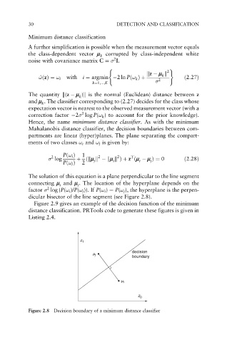
            The solution of this equation is a plane perpendicular to the line segment
            connecting m and m . The location of the hyperplane depends on the
                              j
                        i
                   2
            factor   log (P(! i )/P(! j )). If P(! i ) ¼ P(! j ), the hyperplane is the perpen-
            dicular bisector of the line segment (see Figure 2.8).
              Figure 2.9 gives an example of the decision function of the minimum
            distance classification. PRTools code to generate these figures is given in
            Listing 2.4.
                               z 1
                                    µ              decision
                                     j
                                                   boundary


                                               µ i


                                                     z 0

            Figure 2.8  Decision boundary of a minimum distance classifier
   36   37   38   39   40   41   42   43   44   45   46