
Page 43 - Classification Parameter Estimation & State Estimation An Engg Approach Using MATLAB
P. 43
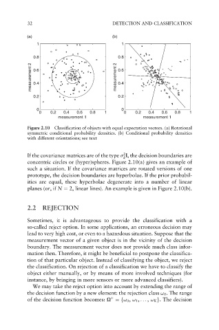
32                               DETECTION AND CLASSIFICATION


            (a)                              (b)
               1                                 1


              0.8                              0.8
             measurement 2   0.6               measurement 2   0.6


              0.4
                                               0.4
              0.2                              0.2

               0                                 0
                0    0.2  0.4  0.6  0.8   1       0   0.2  0.4  0.6   0.8  1
                        measurement 1                    measurement 1

            Figure 2.10  Classification of objects with equal expectation vectors. (a) Rotational
            symmetric conditional probability densities. (b) Conditional probability densities
            with different orientations; see text


                                                 2
            If the covariance matrices are of the type   I, the decision boundaries are
                                                 k
            concentric circles or (hyper)spheres. Figure 2.10(a) gives an example of
            such a situation. If the covariance matrices are rotated versions of one
            prototype, the decision boundaries are hyperbolae. If the prior probabil-
            ities are equal, these hyperbolae degenerate into a number of linear
            planes (or, if N ¼ 2, linear lines). An example is given in Figure 2.10(b).


            2.2   REJECTION


            Sometimes, it is advantageous to provide the classification with a
            so-called reject option. In some applications, an erroneous decision may
            lead to very high cost, or even to a hazardous situation. Suppose that the
            measurement vector of a given object is in the vicinity of the decision
            boundary. The measurement vector does not provide much class infor-
            mation then. Therefore, it might be beneficial to postpone the classifica-
            tion of that particular object. Instead of classifying the object, we reject
            the classification. On rejection of a classification we have to classify the
            object either manually, or by means of more involved techniques (for
            instance, by bringing in more sensors or more advanced classifiers).
              We may take the reject option into account by extending the range of
            the decision function by a new element: the rejection class ! 0 . The range
                                            þ
            of the decision function becomes: O ¼f! 0 , ! 1 , ... , ! K g. The decision