
Page 60 - Classification Parameter Estimation & State Estimation An Engg Approach Using MATLAB
P. 60
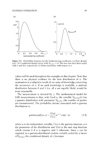
BAYESIAN ESTIMATION                                           49


             (a)                                (b)
               2.5                              1.5
                                                   x p(z|x)
             p(x)
                2

                                                 1          N probes =8
               1.5

                1
                                                0.5
               0.5


                0                                0
                 0   0.2  0.4  0.6  0.8 x  1      0  0.5  1   1.5  2  2.5  3
                     backscattering coefficient                         z/x
            Figure 3.4 Probability densities for the backscattering coefficient. (a) Prior density
            p(x). (b) Conditional density p(zjx) with N probes ¼ 8. The two axes have been scaled
            with x and 1/x, respectively, to obtain invariance with respect to x


              values will be used throughout the examples in this chapter. Note that
              there is no physical evidence for the beta distribution of x. The
              assumption is a subjective result of our state of knowledge concerning
              the occurrence of x. If no such knowledge is available, a uniform
              distribution between 0 and 1 (i.e. all x are equally likely) would be
              more reasonable.
                The measurement is denoted by z. The mathematical model for
              SAR measurements is that, with fixed x, the variable N probes z/x has
              a gamma distribution with parameter N probes (the number of probes
              per measurement). The probability density associated with a gamma
              distribution is:


                                             UðuÞ    1
                          gamma pdfðu; Þ¼        u    expð uÞ           ð3:4Þ
                                              ð Þ

              where u is the independent variable,  ( ) is the gamma function, a is
              the parameter of the distribution and U(u) is the unit step function
              which returns 0 if u is negative and 1 otherwise. Since z can be
              regarded as a gamma-distributed random variable scaled by a factor
              x/N probes , the conditional density of z becomes: