
Page 58 - Classification Parameter Estimation & State Estimation An Engg Approach Using MATLAB
P. 58
BAYESIAN ESTIMATION 47
1
coefficient and its corresponding measurement. In this example, the
number of probes per measurement is eight. It can be seen that, even
after averaging, the measurement is still inaccurate. Moreover,
although the true backscattering coefficient is always between 0 and 1,
the measurements can easily violate this constraint (some measure-
ments are greater than 1).
The task of a parameter estimator here is to map each measurement
to an estimate of the corresponding backscattering coefficient.
This chapter addresses the problem of how to design a parameter
estimator. For that, two approaches exist: Bayesian estimation (Section
3.1) and data-fitting techniques (Section 3.3). The Bayesian-theoretic
framework for parameter estimation follows the same line of reasoning
as the one for classification (as discussed in Chapter 2). It is a probabil-
istic approach. The second approach, data fitting, does not have such a
probabilistic context. The various criteria for the evaluation of an esti-
mator are discussed in Section 3.2.
3.1 BAYESIAN ESTIMATION
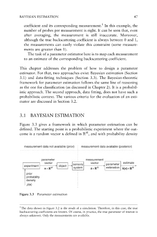
Figure 3.3 gives a framework in which parameter estimation can be
defined. The starting point is a probabilistic experiment where the out-
M
come is a random vector x defined in R , and with probability density
measurement data not available (prior) measurement data available (posterior)
parameter measurement
vector vector estimate
experiment object sensory parameter
x ∈R M system z ∈R N estimation ˆ x(z) ∈R M
prior
probability
density
p(x)
Figure 3.3 Parameter estimation
1
The data shown in Figure 3.2 is the result of a simulation. Therefore, in this case, the true
backscattering coefficients are known. Of course, in practice, the true parameter of interest is
always unknown. Only the measurements are available.