Page 64 - Classification Parameter Estimation & State Estimation An Engg Approach Using MATLAB

BAYESIAN ESTIMATION 53

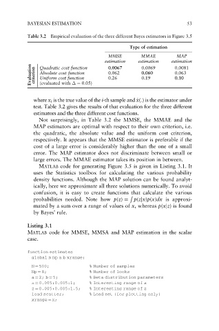
Table 3.2 Empirical evaluation of the three different Bayes estimators in Figure 3.5

Type of estimation
MMSE MMAE MAP
estimation estimation estimation
Evaluation criterion Quadratic cost function 0.0067 0.0069 0.0081
0.063
0.062
0.060
Absolute cost function
Uniform cost function
0.10
0.19
0.26
(evaluated with ¼ 0:05)
x
where x i is the true value of the i-th sample and ^ x(:) is the estimator under
test. Table 3.2 gives the results of that evaluation for the three different
estimators and the three different cost functions.
Not surprisingly, in Table 3.2 the MMSE, the MMAE and the
MAP estimators are optimal with respect to their own criterion, i.e.
the quadratic, the absolute value and the uniform cost criterion,
respectively. It appears that the MMSE estimator is preferable if the
cost of a large error is considerably higher than the one of a small
error. The MAP estimator does not discriminate between small or
large errors. The MMAE estimator takes its position in between.
MATLAB code for generating Figure 3.5 is given in Listing 3.1. It
uses the Statistics toolbox for calculating the various probability
density functions. Although the MAP solution can be found analyt-
ically, here we approximate all three solutions numerically. To avoid
confusion, it is easy to create functions that calculate the various
R
probabilities needed. Note how p(z) ¼ p(zjx)p(x)dx is approxi-
mated by a sum over a range of values of x, whereas p(xjz) is found
by Bayes’ rule.

Listing 3.1
MATLAB code for MMSE, MMSA and MAP estimation in the scalar
case.

function estimates
global N Np a b xrange;
N ¼ 500; % Number of samples
Np ¼ 8; % Number of looks
a ¼ 2; b ¼ 5; % Beta distribution parameters
x ¼ 0.005:0.005:1; % Interesting range of x
z ¼ 0.005:0.005:1.5; % Interesting range of z
load scatter; % Load set (for plotting only)
xrange ¼ x;