Page 67 - Classification Parameter Estimation & State Estimation An Engg Approach Using MATLAB
P. 67
56 PARAMETER ESTIMATION
3.1.3 The Gaussian case with linear sensors
Suppose that the parameter vector x has a normal distribution with
expectation vector E[x] ¼ m and covariance matrix C x . In addition,
x
suppose that the measurement vector can be expressed as a linear
combination of the parameter vector corrupted by additive Gaussian
noise:
z ¼ Hx þ v ð3:18Þ
where v is an N-dimensional random vector with zero expectation and
covariance matrix C v . x and v are uncorrelated. H is an N M matrix.
The assumption that both x and v are normal implies that the condi-
tional probability density of z is also normal. The conditional expect-
ation vector of z equals:
E½zjx¼ m ¼ Hm
zjx x ð3:19Þ
The conditional covariance matrix of z is C zjx ¼ C v .
Under these assumptions the posterior distribution of x is normal as
well. Application of (3.2) yields the following expressions for the MMSE
estimate and the corresponding covariance matrix:
1
1
1
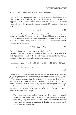
^ x x MMSE ðzÞ¼ m ¼ E½xjz¼ H C H þ C 1 1 H C z þ C m
T
T
xjz v x v x x
T
1
C xjz ¼ H C H þ C 1 1
v x
ð3:20Þ
The proof is left as an exercise for the reader. See exercise 3. Note that
m , being the posterior expectation, is the MMSE estimate ^ x MMSE (z).
x
xjz
The posterior expectation, E[xjz], consists of two terms. The first term
is linear in z. It represents the information coming from the measure-
ment. The second term is linear in m , representing the prior knowledge.
x
To show that this interpretation is correct it is instructive to see what
happens at the extreme ends: either no information from the measure-
ment, or no prior knowledge:
. The measurements are useless if the matrix H is virtually zero, or if
the noise is too large, i.e. C 1 is too small. In both cases, the second
v
term in (3.20) dominates. In the limit, the estimate becomes
^ x x MMSE (z) ¼ m with covariance matrix C x , i.e. the estimate is purely
x
based on prior knowledge.

