Page 95 - Classification Parameter Estimation & State Estimation An Engg Approach Using MATLAB

84 STATE ESTIMATION

The probability of x(i þ 1) depends solely on x(i) and not on the past
states. In order to predict x(i þ 1), the knowledge of the full history is
not needed. It suffices to know the present state. If the Markov condition
applies, the state of a physical process is a summary of the history of the
process.

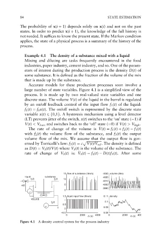
Example 4.1 The density of a substance mixed with a liquid
Mixing and diluting are tasks frequently encountered in the food
industries, paper industry, cement industry, and so. One of the param-
eters of interest during the production process is the density D(t)of
some substance. It is defined as the fraction of the volume of the mix
that is made up by the substance.
Accurate models for these production processes soon involve a
large number of state variables. Figure 4.1 is a simplified view of the
process. It is made up by two real-valued state variables and one
discrete state. The volume V(t) of the liquid in the barrel is regulated
by an on/off feedback control of the input flow f 1 (t) of the liquid:
f 1 (t) ¼ f 0 x(t). The on/off switch is represented by the discrete state
variable x(t) 2f0,1g. A hysteresis mechanism using a level detector
(LT) prevents jitter of the switch. x(t) switches to the ‘on’ state (¼1) if
V(t) < V low , and switches back to the ‘off’ state (¼0) if V(t) > V high .
_
The rateofchangeof thevolume is V(t) ¼ f 1 (t) þ f 2 (t) f 3 (t)
V
with f 2 (t) the volume flow of the substance, and f 3 (t) the output
volume flow of the mix. We assume that the output flow is gov-
erned by Torricelli’s law: f 3 (t) ¼ c V(t)/V ref . The density is defined
p
ffiffiffiffiffiffiffiffiffiffiffiffiffiffiffiffiffiffiffi
as D(t) ¼ V S (t)/V(t)where V S (t) is the volume of the substance. The
_
V
rate of change of V S (t)is: V S (t) ¼ f 2 (t) D(t)f 3 (t). After some

15 flow of substance (litre/s) 4030 volume (litre)
liquid substance 4020
f (t) f (t) 10
1 2
4010
x(t) 5 4000
3990
0
LT
1.5 liquid input flow (litre/s) 0.11 density
V(t),D(t) 1
f (t) 0.1
3
0.5
DT 0.09
0
–0.5 0.08
0 2000 4000 0 2000 400
i∆ (s) i∆ (s)
Figure 4.1 A density control system for the process industry