Page 98 - Classification Parameter Estimation & State Estimation An Engg Approach Using MATLAB

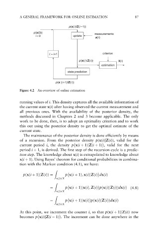
A GENERAL FRAMEWORK FOR ONLINE ESTIMATION 87

p(x(i)|Z(i–1))
p(x(0)) measurements
i = 0 update
z(i )

i:= i+1 criterion
p(x(i)|Z(i)) ˆ x(i)
estimation
state prediction

p(x (i+1)|Z(i))
Figure 4.2 An overview of online estimation

running values of i. This density captures all the available information of
the current state x(i) after having observed the current measurement and
all previous ones. With the availability of the posterior density, the
methods discussed in Chapters 2 and 3 become applicable. The only
work to be done, then, is to adopt an optimality criterion and to work
this out using the posterior density to get the optimal estimate of the
current state.
The maintenance of the posterior density is done efficiently by means
of a recursion. From the posterior density p(x(i)jZ(i)), valid for the

current period i, the density p x(i þ 1)jZ(i þ 1) , valid for the next
period i þ 1, is derived. The first step of the recursion cycle is a predic-
tion step. The knowledge about x(i) is extrapolated to knowledge about
x(i þ 1). Using Bayes’ theorem for conditional probabilities in combina-
tion with the Markov condition (4.1), we have:

Z

pðxði þ 1ÞjZðiÞÞ ¼ p xði þ 1Þ; xðiÞjZðiÞ dxðiÞ
xðiÞ2X
Z

¼ p xði þ 1ÞjxðiÞ; ZðiÞ pðxðiÞjZðiÞÞdxðiÞ ð4:8Þ
xðiÞ2X
Z

¼ p xði þ 1ÞjxðiÞ pðxðiÞjZðiÞÞdxðiÞ
xðiÞ2X
At this point, we increment the counter i, so that p(x(i þ 1)jZ(i)) now
becomes p x(i)jZ(i 1) . The increment can be done anywhere in the