Page 96 - Classification Parameter Estimation & State Estimation An Engg Approach Using MATLAB

A GENERAL FRAMEWORK FOR ONLINE ESTIMATION 85

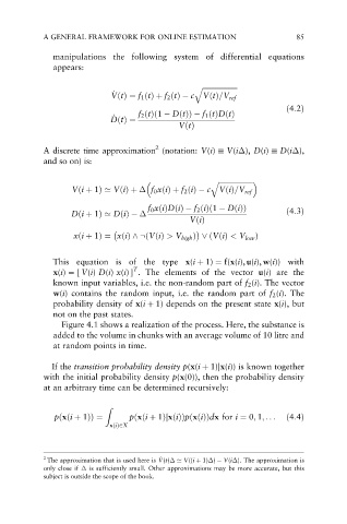
manipulations the following system of differential equations
appears:

q ffiffiffiffiffiffiffiffiffiffiffiffiffiffiffiffiffiffiffiffi
_
V VðtÞ¼ f 1 ðtÞþ f 2 ðtÞ c VðtÞ=V ref
ð4:2Þ
_ f 2 ðtÞð1 DðtÞÞ f 1 ðtÞDðtÞ
D DðtÞ¼
VðtÞ
2
A discrete time approximation (notation: V(i) V(i ), D(i) D(i ),
and so on) is:

q ffiffiffiffiffiffiffiffiffiffiffiffiffiffiffiffiffiffiffiffi
Vði þ 1Þ’ VðiÞþ f 0 xðiÞþ f 2 ðiÞ c VðiÞ=V ref

f 0 xðiÞDðiÞ f 2 ðiÞð1 DðiÞÞ
Dði þ 1Þ’ DðiÞ ð4:3Þ
VðiÞ

xði þ 1Þ¼ xðiÞ^:ðVðiÞ > V high Þ _ðVðiÞ < V low Þ

This equation is of the type x(i þ 1) ¼ f(x(i), u(i), w(i)) with
T
x(i) ¼ [ V(i) D(i) x(i)] . The elements of the vector u(i) are the
known input variables, i.e. the non-random part of f 2 (i). The vector
w(i) contains the random input, i.e. the random part of f 2 (i). The
probability density of x(i þ 1) depends on the present state x(i), but
not on the past states.
Figure 4.1 shows a realization of the process. Here, the substance is
added to the volume in chunks with an average volume of 10 litre and
at random points in time.

If the transition probability density p(x(i þ 1)jx(i)) is known together
with the initial probability density p(x(0)), then the probability density
at an arbitrary time can be determined recursively:

Z
pðxði þ 1ÞÞ ¼ pðxði þ 1ÞjxðiÞÞpðxðiÞÞdx for i ¼ 0; 1; .. . ð4:4Þ
xðiÞ2X

2 _
The approximation that is used here is V(t) ’ V((i þ 1) ) V(i ). The approximation is
V
only close if is sufficiently small. Other approximations may be more accurate, but this
subject is outside the scope of the book.