Page 108 - Complementarity and Variational Inequalities in Electronics

A Variational Inequality Theory Chapter | 4 99

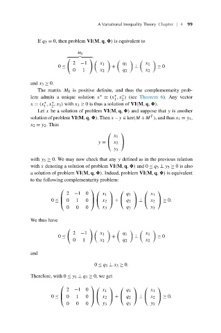
If q 3 = 0, then problem VI(M,q, ) is equivalent to

M 0

2 −1 x 1 q 1 x 1
0 ≤ + ⊥ ≥ 0
0 1 x 2 q 2 x 2
and x 3 ≥ 0.
The matrix M 0 is positive definite, and thus the complementarity prob-
∗
∗
lem admits a unique solution x = (x ,x ) (see Theorem 6). Any vector
∗
1 2
x = (x ,x ,x 3 ) with x 3 ≥ 0 is thus a solution of VI(M,q, ).
∗
∗
1 2
Let x be a solution of problem VI(M,q, ) and suppose that y is another
T
solution of problem VI(M,q, ). Then x−y ∈ ker(M +M ), and thus x 1 = y 1 ,
x 2 = y 2 . Thus
⎛ ⎞
x 1
y = ⎝ x 2 ⎠
y 3
with y 3 ≥ 0. We may now check that any y defined as in the previous relation
with x denoting a solution of problem VI(M,q, ) and 0 ≤ q 3 ⊥ y 3 ≥ 0is also
a solution of problem VI(M,q, ). Indeed, problem VI(M,q, ) is equivalent
to the following complementarity problem:

⎛ ⎞ ⎛ ⎞ ⎛ ⎞ ⎛ ⎞
2 −10 x 1 q 1 x 1
0 ≤ ⎝ 0 1 0 ⎠ ⎝ x 2 ⎠ + ⎝ q 2 ⎠ ⊥ ⎝ x 2 ⎠ ≥ 0.
⎟
⎜
0 0 0 x 3 q 3 x 3
We thus have

2 −1 x 1 q 1 x 1
0 ≤ + ⊥ ≥ 0
0 1 x 2 q 2 x 2
and

0 ≤ q 3 ⊥ x 3 ≥ 0.

Therefore, with 0 ≤ y 3 ⊥ q 3 ≥ 0, we get
⎛ ⎞ ⎛ ⎞ ⎛ ⎞ ⎛ ⎞
2 −10 x 1 q 1 x 1
0 ≤ ⎝ 0 1 0 ⎠ ⎝ x 2 ⎠ + ⎝ q 2 ⎠ ⊥ ⎝ x 2 ⎠ ≥ 0.
⎜
⎟
0 0 0 y 3 q 3 y 3