Page 160 - Complementarity and Variational Inequalities in Electronics

The Nonregular Dynamical System Chapter | 5 151

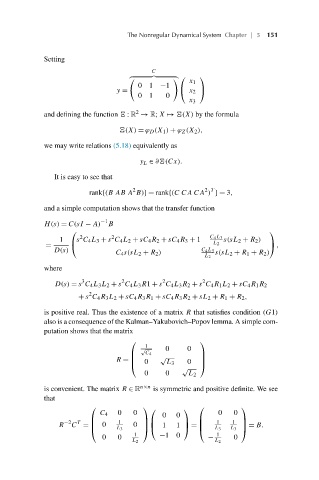
Setting
C

⎛ ⎞
x 1
01 −1
y = ⎝ x 2 ⎠
01 0
x 3
2
and defining the function : R → R;X → (X) by the formula
(X) = ϕ D (X 1 ) + ϕ Z (X 2 ),

we may write relations (5.18) equivalently as

y L ∈ ∂ (Cx).
It is easy to see that

2
2 T
rank{(B AB A B)}= rank{(C CA CA ) }= 3,
and a simple computation shows that the transfer function
H(s) = C(sI − A) −1 B
⎛ ⎞
2
2
1 s C 4 L 3 + s C 4 L 2 + sC 4 R 2 + sC 4 R 3 + 1 C 4 L 3 s(sL 2 + R 2 )
L 2
= ⎝ ⎠ ,
D(s) C 4 s(sL 2 + R 2 ) C 4 L 3 s(sL 2 + R 1 + R 2 )
L 2
where
3 2 2 2
D(s) = s C 4 L 3 L 2 + s C 4 L 3 R1 + s C 4 L 3 R 2 + s C 4 R 1 L 2 + sC 4 R 1 R 2
2
+ s C 4 R 3 L 2 + sC 4 R 3 R 1 + sC 4 R 3 R 2 + sL 2 + R 1 + R 2 ,
is positive real. Thus the existence of a matrix R that satisfies condition (G1)
also is a consequence of the Kalman–Yakubovich–Popov lemma. A simple com-
putation shows that the matrix

⎛ ⎞
1
√ 0 0
C 4
√
⎜ ⎟
R = ⎜ 0 L 3 0 ⎟
⎝ ⎠
√
0 0 L 2
is convenient. The matrix R ∈ R n×n is symmetric and positive definite. We see
that
⎛ ⎞ ⎛ ⎞ ⎛ ⎞
C 4 0 0 0 0 0 0
−2 T ⎜ 1 ⎟ ⎜ ⎟ ⎜ 1 1 ⎟
⎜ 0
R C = 0 ⎟ ⎝ 1 1 ⎠ = ⎜ ⎟ = B.
L 3 L 3
⎝ ⎠ ⎝ L 3 ⎠
0 0 1 −10 − 1 0
L 2 L 2