Page 130 - Computational Colour Science Using MATLAB

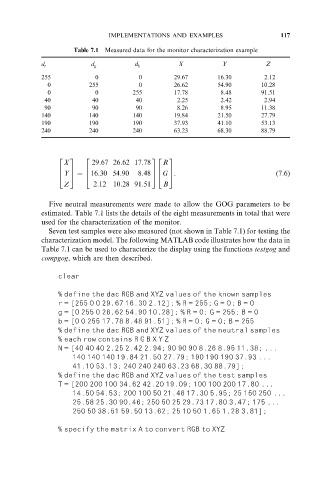
IMPLEMENTATIONS AND EXAMPLES 117

Table 7.1 Measured data for the monitor characterization example
X Y Z
d r d g d b
255 0 0 29.67 16.30 2.12
0 255 0 26.62 54.90 10.28
0 0 255 17.78 8.48 91.51
40 40 40 2.25 2.42 2.94
90 90 90 8.26 8.95 11.38
140 140 140 19.84 21.50 27.79
190 190 190 37.93 41.10 53.13
240 240 240 63.23 68.30 88.79

2 3 2 32 3
X 29:67 26:62 17:78 R
16:30 54:90 8:48 5 G 5.
6 7 6 76 7
4 Y 5 ¼ 4 4 ð7:6Þ
Z 2:12 10:28 91:51 B
Five neutral measurements were made to allow the GOG parameters to be
estimated. Table 7.1 lists the details of the eight measurements in total that were
used for the characterization of the monitor.
Seven test samples were also measured (not shown in Table 7.1) for testing the
characterization model. The following MATLAB code illustrates how the data in
Table 7.1 can be used to characterize the display using the functions testgog and
compgog, which are then described.

clear

% define the dac RGB and XYZ values of the known samples
r = [255 0 0 29.67 16.30 2.12]; % R = 255; G = 0; B = 0
g = [0 255 0 26.62 54.90 10.28]; % R = 0; G = 255; B = 0
b = [0 0 255 17.78 8.48 91.51]; % R = 0; G = 0; B = 255
% define the dac RGB and XYZ values of the neutral samples
% each row contains R G B X Y Z
N = [40 40 40 2.25 2.42 2.94; 90 90 90 8.26 8.95 11.38; ...
140 140 140 19.84 21.50 27.79; 190 190 190 37.93 ...
41.10 53.13; 240 240 240 63.23 68.30 88.79];
% define the dac RGB and XYZ values of the test samples
T = [200 200 100 34.62 42.20 19.09; 100 100 200 17.80 ...
14.50 54.53; 200 100 50 21.46 17.30 5.95; 25 150 250 ...
25.58 25.30 90.46; 250 50 25 29.73 17.80 3.47; 175 ...
250 50 38.51 59.50 13.62; 25 10 50 1.65 1.28 3.81];

% specify the matrix A to convert RGB to XYZ