Page 172 - Computational Colour Science Using MATLAB

IMPLEMENTATIONS AND EXAMPLES 159

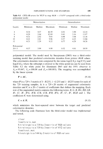
Table 9.1 CIELAB errors for MLP to map RGB ! L*a*b* compared with a third-order
polynomial model
Memorization Generalization

Layers Minimum Median Maximum Minimum Median Maximum

4 0.34 4.37 16.59 0.41 3.90 12.14
6 0.28 3.84 12.89 0.41 3.16 11.87
8 0.31 2.92 9.43 0.44 3.84 11.36
10 0.21 2.81 9.96 0.37 4.23 11.04
12 0.21 2.29 9.32 0.77 4.29 10.28
Polynomial
2063 0.37 3.99 9.99 0.52 4.01 10.59

polynomial model. The model used by Sueeprasan (2003) was a third-order
masking model that predicted colorimetric densities from printer RGB values.
The colorimetric densities were computed by the terms log(X/X ), log(Y/Y ) and
n
n
log(Z/Z ), where the subscript n referred to the white point (as can be seen from
n
Table 4.2 the white point for illuminant D65 and the 1931 observer is
X ¼ 95.047, Y ¼ 100.00 and Z ¼ 108.883). The mapping was accomplished
n
n
n
by the linear system
P ¼ AC, ð9:14Þ
where P is a 72963 matrix of 1 R/255, 1 G/255 and 1 B/255 terms for each of
the 729 training samples, A is a 729620 matrix of augmented colorimetic
densities and C is a 2063 matrix of coefficients that defines the mapping. Each
row of the augmented matrix contains the following terms: R, G, B, RG, RB, GB,
2
2
2
3
3
3
2
2
2
2
R , G , B , R G, R B, G R, G B, B R, B G, R , G , B , RGB and 1. The
2
2
coefficients C were determined using
C ¼ A P, ð9:15Þ
þ
which minimizes the least-squared error between the target and predicted
colorimetric densities.
The following code illustrates how the third-order model was implemented
and tested,
clear
load train.mat
% trainrgb is a 729 by 3 matrix of RGB values
% trainxyz is a 729 by 3 matrix of XYZ values
load test.mat
% testrgb is a 144 by 3 matrix of RGB values