
Page 170 - Computational Colour Science Using MATLAB
P. 170
IMPLEMENTATIONS AND EXAMPLES 157
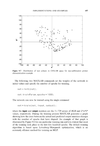
Figure 9.7 Distribution of test colours in CIELAB space for dye-sublimation printer
characterization example
The following two MATLAB commands set the weights of the network to
initial values and specify the number of epochs for training,
net = init(net);
net.trainParam.epochs = 1000;
The network can now be trained using the single command
net = train(net, input, output);
where the input and output matrices are the 36729 arrays of RGB and L*a*b*
values, respectively. During the training process MATLAB generates a graph
showing how the error between the actual and predicted output matrices changes
with the number of epochs that have elapsed. An example of that graph is
illustrated by Figure 9.8 for one particular training run and it is evident that most
of the training took place in the first few hundred epochs. The default training
algorithm is based upon Levenberg–Marquardt optimization, which is an
extremely efficient method for training an MLP.