
Page 166 - Computational Colour Science Using MATLAB
P. 166
IMPLEMENTATIONS AND EXAMPLES 153
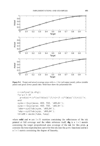
Figure 9.4 Target and actual coverage areas with n ¼ 1 for red (upper panel), yellow (middle
panel) and green (lower panel) inks. Solid lines show the polynomial fits
c = polyval(p,dig);
for w = 1:31
pred(w) = (c*(solid(w))^(1/n)+(1-c)*(W(w)^(1/n)))^n;
end
xyzm = r2xyz(meas, 400, 700, ’d65___64’);
xyzp = r2xyz(pred, 400, 700, ’d65___64’);
labm = xyz2lab(xyzm, ’d65___64’);
labp = xyz2lab(xyzp, ’d65___64’);
thisDE = cmcde(labm, labp)
where solid and w are 1631 matrices containing the reflectances of the ink
printed at full coverage and the white substrate itself, dig is a 161 matrix
containing the target proportional area coverage of the ink for this print, p
contains the tone-reproduction curve for this ink (see the gettrc function) and n is
a161 matrix containing the degree of linearity.