Page 187 - Computational Colour Science Using MATLAB

174 MULTISPECTRAL IMAGING

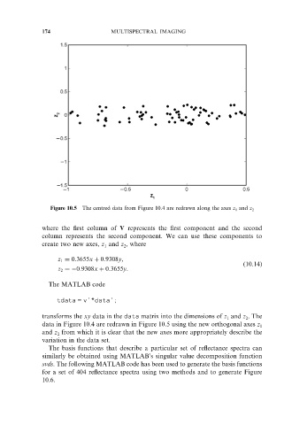
Figure 10.5 The centred data from Figure 10.4 are redrawn along the axes z 1 and z 2

where the first column of V represents the first component and the second
column represents the second component. We can use these components to
create two new axes, z and z , where
2
1
z 1 ¼ 0:3655x þ 0:9308y,
ð10.14Þ
z 2 ¼ 0:9308x þ 0:3655y.
The MATLAB code

tdata = v’*data’;

transforms the xy data in the data matrix into the dimensions of z and z . The
1
2
data in Figure 10.4 are redrawn in Figure 10.5 using the new orthogonal axes z 1
and z from which it is clear that the new axes more appropriately describe the
2
variation in the data set.
The basis functions that describe a particular set of reflectance spectra can
similarly be obtained using MATLAB’s singular value decomposition function
svds. The following MATLAB code has been used to generate the basis functions
for a set of 404 reflectance spectra using two methods and to generate Figure
10.6.