
Page 255 - Computational Fluid Dynamics for Engineers
P. 255
8.1 Introduction 245
0.25
-
0.20 0.100 / ai = 0
^ / / =-0.004
"^^C^- = -0.006
! X X J S I s ^ , = -0.007
0.15 ^ \ \ ^ ^ ^ v ^ =-0.0075
a r
0.10 0.010
!
0.05
0.00 J H J J
10 io io io 1(T 10 10 io
R R
(a) (b)
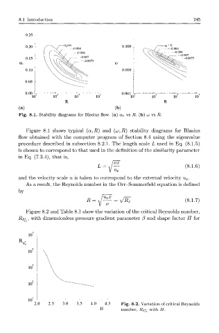
Fig. 8.1. Stability diagrams for Blasius flow, (a) a r vs R. (b) u vs R.
Figure 8.1 shows typical (a, R) and (a;, R) stability diagrams for Blasius
flow obtained with the computer program of Section 8.4 using the eigenvalue
procedure described in subsection 8.2.1. The length scale L used in Eq. (8.1.5)
is chosen to correspond to that used in the definition of the similarity parameter
in Eq. (7.3.4), that is,
L=M (8.1.6)
u
V e
and the velocity scale u is taken to correspond to the external velocity u e.
As a result, the Reynolds number in the Orr-Sommerfeld equation is defined
by
U eX r—
R — \l — — v Rx (8.1.7)
Figure 8.2 and Table 8.1 show the variation of the critical Reynolds number,
R$* , with dimensionless pressure gradient parameter (3 and shape factor H for
10
R.
10
io J
10
10
2.0 2.5 3.0 3.5 4.0 4.5 Fig. 8.2. Variation of critical Reynolds
H number, R$* with H.