Page 258 - Computational Fluid Dynamics for Engineers

248 8. Stability and Transition

where now
C3 ci = £1, c 4 = £ 2 (8.2.6)
6 + 6'
The difference equations (8.2.3) and (8.2.5) have trivial solutions fj = Sj = (f)j —
gj = 0 for all j and we shall use the iteration procedure described below to find
the special parameter values for which nontrivial solutions exist.
Since the Orr-Sommerfeld equation and the boundary conditions are ho-
mogenous, the trivial solution (f)(y) = 0 is valid for all values of a, /?, uo and R. For
this reason to compute the eigenvalues and the eigenfunctions we first replace
the boundary condition 0'(O) = 0 (that is f 0 = 0) of Eq. (8.2.5) by 0"(O) = 1,
that is so = 1. Now the difference equations have a non-trivial solution since
^"(O) 7^ 0 and we seek to adjust or to determine parameter values so that the
original boundary condition is satisfied. This is achieved by an iteration scheme
based on Newton's method. Specifically, we first write the wall boundary con-
ditions
0o = (ri)o = O, so = (r 2 )o = l (8.2.7)
and the edge boundary conditions in Eq. (8.2.5b) and Eq. (8.2.3) in matrix-
vector form as in Eq. (4.4.29), with Sj and fj defined by

4>j (nh
S J
*; = . f J = (8.2.
h
9j
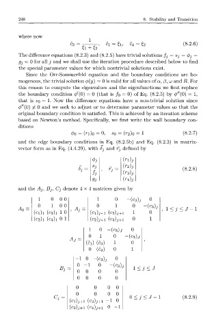
and the Aj, Bj^ Cj denote 4 4 matrices given by

1 0 0 0 1 0 -{c 3)j 0
0 1 0 0 0 1 0 -(c 3)j
= , Aj —
A 0 1 < j < J
(ci)i (c 3 )i 1 0 (Cl)j+1 (C3)i+1 1 0
(C2)i (c 4 )i 0 1 (C2)j+1 (C4)j + 1 0 1
1 0 -{c z)j 0
0 1 0 "(C3)j
Aj =
(ci) (cs) 1 0
0 (c 4) 0 1
- 1 0 -(c 3 )j 0
c
0 - 1 0 "( s)i
Bj = 1 < 3 < J
0 0 0 0
0 0 0 0
0 0 0 0
0 0 0 0
= 0 < j < J - 1 (8.2.9)
c 3
(ci)j+i (c 3 )i+i - 1 0
(c 2 )i+i (c 4 ) J + i 0 - 1