Page 262 - Computational Fluid Dynamics for Engineers

252 8. Stability and Transition

(r 3l sj J.2.21c)

- _ f dd4
(rt)j = sj (8.2.21d)
\dR
As before, with the coefficient matrix A already known, we now compute the
relations in Eqs. (8.2.21) so that df/dR can be obtained from the solution of
Eq. (8.2.20). Since df/da r and df/dou are already known from the solutions
of Eqs. (8.2.15), da r/dR and duo/dR can be computed from Eqs. (8.2.19) to
decide on the choice of the eigenvalue procedure.
It should be mentioned that the values of da r/dR and du/dR can also be
very useful in estimating the initial values of a r and a; at a different Reynolds
number where new sets of a r and u are to be obtained. To discuss this point
further, we expand a r and u by Taylor's series and by retaining only the first
term, we write

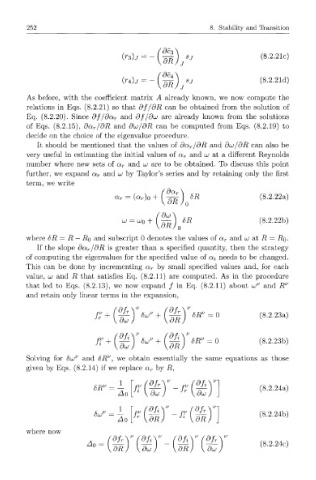
— (a r)o + 3.2.22a)
a r

(8.2.22b)
W O +
( ^ ) o ^
where 6R = R — RQ and subscript 0 denotes the values of a r and u at R = RQ.
If the slope da r/dR is greater than a specified quantity, then the strategy
of computing the eigenvalues for the specified value of oti needs to be changed.
This can be done by incrementing a r by small specified values and, for each
value, UJ and R that satisfies Eq. (8.2.11) are computed. As in the procedure
that led to Eqs. (8.2.13), we now expand / in Eq. (8.2.11) about u u and R v
and retain only linear terms in the expansion,
+
v
du ^ (i) =° (8.2.23a)
Jr +
'
v+
+
'• <f) (I)^=° 3.2.23b)
V
Solving for 8UJ V and 8R , we obtain essentially the same equations as those
given by Eqs. (8.2.14) if we replace a r by R,

bR v = \ (8.2.24a)

cufdfrY _ fv{df LY
8LO V (8.2.24b)
Ao
r Ji
where now \dRj \dRj
(8.2.24c)
Q
A = (!MLY (WiY _ (HAY ( JL
0
\dR) \duj) \dRj \du