Page 264 - Computational Fluid Dynamics for Engineers

254 8. Stability and Transition

line3
oc r

® ©

R
n
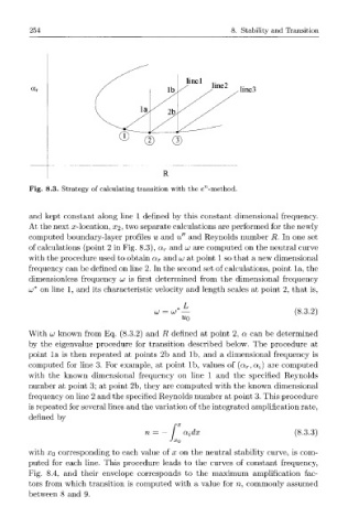
Fig. 8.3. Strategy of calculating transition with the e -method.

and kept constant along line 1 defined by this constant dimensional frequency.
At the next x-location, X2-, two separate calculations are performed for the newly
computed boundary-layer profiles u and v!' and Reynolds number R. In one set
of calculations (point 2 in Fig. 8.3), a r and UJ are computed on the neutral curve
with the procedure used to obtain a r and UJ at point 1 so that a new dimensional
frequency can be defined on line 2. In the second set of calculations, point la, the
dimensionless frequency UJ is first determined from the dimensional frequency
UJ* on line 1, and its characteristic velocity and length scales at point 2, that is,

UJ = UJ (8.3.2)
n 0
With UJ known from Eq. (8.3.2) and R defined at point 2, a can be determined
by the eigenvalue procedure for transition described below. The procedure at
l
l
point a is then repeated at points 2b and b, and a dimensional frequency is
(
l
computed for line 3. For example, at point b, values of a r ,c^) are computed
with the known dimensional frequency on line 1 and the specified Reynolds
number at point 3; at point 2b, they are computed with the known dimensional
frequency on line 2 and the specified Reynolds number at point 3. This procedure
is repeated for several lines and the variation of the integrated amplification rate,
defined by

n / a, dx (8.3.3)
JXQ
with xo corresponding to each value of x on the neutral stability curve, is com-
puted for each line. This procedure leads to the curves of constant frequency,
Fig. 8.4, and their envelope corresponds to the maximum amplification fac-
tors from which transition is computed with a value for n, commonly assumed
between 8 and 9.