Page 265 - Computational Fluid Dynamics for Engineers

n
8.3 e -Method 255

2.0 i -
0.0 - AS

8.0 /j-/
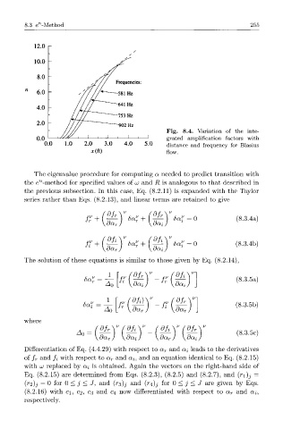
// / Frequencies:
7/ / /
6.0 / / / / / -581 Hz
-641 Hz
4.0
-753 Hz
2.0 —902 Hz
Fig. 8.4. Variation of the inte-
0.0 1 l 1 . I grated amplification factors with
0 0 1.0 2.0 3.0 4.0 5.0 distance and frequency for Blasius
x(ft) flow.

The eigenvalue procedure for computing a needed to predict transition with
n
the e -method for specified values of uu and R is analogous to that described in
the previous subsection. In this case, Eq. (8.2.11) is expanded with the Taylor
series rather than Eqs. (8.2.13), and linear terms are retained to give

3/r dfr_
fr boii 8a" = 0 (8.3.4a)
da r don

fi+ 6ar + 8a" = 0 (8.3.4b)
[dZ) [da-
The solution of these equations is similar to those given by Eq. (8.2.14),

8a" — ~r- h Jr (8.3.5a)
* da J {d ai

8a" — —— r -fi dfr 3.3.5b)
1 r
^ o da r
where
dfr_
A 0 (8.3.5c)
da r dai da r
Differentiation of Eq. (4.4.29) with respect to a r and OLI leads to the derivatives
of f r and fi with respect to a r and a^, and an equation identical to Eq. (8.2.15)
with UJ replaced by oti is obtained. Again the vectors on the right-hand side of
Eq. (8.2.15) are determined from Eqs. (8.2.3), (8.2.5) and (8.2.7), and (n)j =
r
( 2)j = 0 for 0 < j < J, and (rs)j and (7*4)^ for 0 < j < J are given by Eqs.
(8.2.16) with ci, C2, C3 and C4 now differentiated with respect to a r and c^,
respectively.