Page 256 - Computational Fluid Dynamics for Engineers

246 8. Stability and Transition

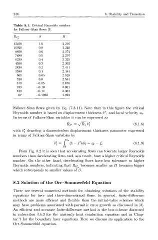
Table 8.1. Critical Reynolds number
for Falkner-Skan flows [3].

% 0 H
12490 1.0 2.216
10920 0.8 2.240
8890 0.6 2.274
7680 0.5 2.297
6230 0.4 2.325
4550 0.3 2.362
2830 0.2 2.411
1380 0.1 2.481
865 0.05 2.529
520 0.0 2.591
318 -0.05 2.676
199 -0.10 2.801
138 -0.14 2.963
67 -0.1988 4.029

Falkner-Skan flows given by Eq. (7.3.11). Note that in this figure the critical
Reynolds number is based on displacement thickness <5*, and local velocity u e.
In terms of Falkner-Skan variables it can be expressed as

Rs* = \fRx6\ (8.1.8)
with 8\ denoting a dimensionless displacement thickness parameter expressed
in terms of Falkner-Skan variables by

*i= r{l-f')dri = rie-fe (8-1.9)
JO
From Fig. 8.2 it is seen that accelerating flows can tolerate larger Reynolds
numbers than decelerating flows and, as a result, have a higher critical Reynolds
number. On the other hand, decelerating flows have less tolerance to higher
Reynolds numbers, indicating that R$* becomes smaller as H becomes bigger
which corresponds to smaller values of (3.

8.2 Solution of the Orr-Sommerfeld Equation

There are several numerical methods for obtaining solutions of the stability
equations for two- and three-dimensional flows. In general, finite-difference
methods are more efficient and flexible than the initial-value schemes which
may have problems associated with parasitic error growth as discussed in [3].
An efficient and accurate finite-difference method is the box-scheme discussed
in subsection 4.4.3 for the unsteady heat conduction equation and in Chap-
ter 7 for the boundary layer equations. Here we discuss its application to the
Orr-Sommerfeld equation.