Page 155 - Computational Modeling in Biomedical Engineering and Medical Physics

144 Computational Modeling in Biomedical Engineering and Medical Physics

Bioimpedance techniques are prominent tools in the noninvasive monitoring of cardiovas-
cular dynamics, which is of great clinical interest. For example, the impedance cardiography
(ICG) is used in conjunction with the ECG (Einthoven’s Triangle & Cardiac Monitoring,
2020) to characterize the mechanical function of the heart, such as stroke volume, left-
ventricular ejection time, cardiac output, or systolic time ratio, of importance in the evaluation
of patients with cardiovascular diseases (Bernstein, 2010; Kubicek et al., 1966; Sramek, 1986).
The pulse wave velocity (PWV) is used to evaluate the arterial stiffness, which is a useful
parameter in arrhythmia diagnosis, hypertension, and stroke events (Lee and Cho, 2015).
Another line of applications is the medical imaging of human body inside, enabled by
the electrical impedance tomography (EIT) (Malmivuo and Plonsey, 1995). An electrode
array placed on the torso provides for boundary voltage measurements that may be used to
find the electrical conductivity distribution (the solution to an inverse problem), hence ana-
tomic structure, which is of great interest, nevertheless, the low resolution still provided.
Numerous reviews, for example, work by Bera (2014), Cicho˙ z-Lach and Michalak
(2017), Ward (2019), Di Vincenzo et al. (2019), Kyle et al. (2004), Kriˇ zaj (2018),prove that
the bioimpedance concept, model, method, and implementation in systems, equipments,
and devices are part commonly used in the biomedical practice. The advantages that distin-
guish the bioimpedance techniques (noninvasive, low-cost, portable, user-friendly) are key
to their rapid acceptance. Their development though has still to overcome significant chal-
lenges, such as miniaturization, efficient algorithms, new parameters, novel sensing technolo-
gies, increased sensitivity, reduced power consumption, improved circuit designs, etc.

5.2 The electrical impedance
Lumped parameters may be defined for boundary value problems without internal sources
when the interaction with the surroundings occurs through ports on the boundary, in a
gradient-flux context, as the ratio between driving gradients and the conjugated fluxes.
For example, for a system where the electromagnetic field interaction with the surround-
ings occurs at two terminals (ports) level only (the electromagnetic field is contained in the
system, does not “cross” the boundary), an electric impedance is calculated as the ratio of
voltage drop (gradient), U(t), over the electric current (flux), I(t), that is, Z(t) 5 U/I
[Ω]—although U and I are not with respect to the same terminals.
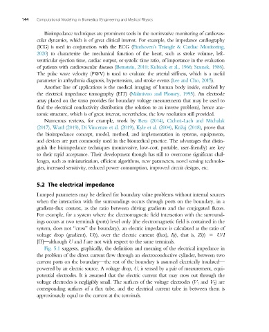
Fig. 5.1 suggests, graphically, the definition and meaning of the electrical impedance in
the problem of the direct current flow through an electroconductive cylinder, between two
current ports on the boundary—the rest of the boundary is assumed electrically insulated—
powered by an electric source. A voltage drop, U, is sensed by a pair of measurement, equi-
potential electrodes. It is assumed that the electric current that may cross out through the
voltage electrodes is negligibly small. The surfaces of the voltage electrodes (V 1 and V 2 )are
corresponding surfaces of a flux tube, and the electrical current tube in between them is
approximately equal to the current at the terminals.