Page 156 - Computational Modeling in Biomedical Engineering and Medical Physics

Bioimpedance methods 145

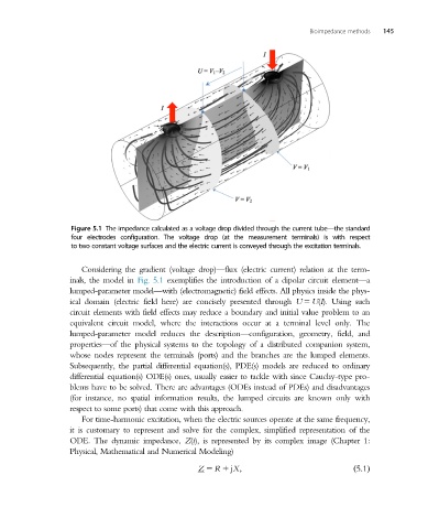
Figure 5.1 The impedance calculated as a voltage drop divided through the current tube—the standard
four electrodes configuration. The voltage drop (at the measurement terminals) is with respect
to two constant voltage surfaces and the electric current is conveyed through the excitation terminals.

Considering the gradient (voltage drop)—flux (electric current) relation at the term-
inals, the model in Fig. 5.1 exemplifies the introduction of a dipolar circuit element—a
lumped-parameter model—with (electromagnetic) field effects. All physics inside the phys-
ical domain (electric field here) are concisely presented through U5 U(I). Using such
circuitelementswithfield effectsmay reduce a boundary and initial value problem to an
equivalent circuit model, where the interactions occur at a terminal level only. The
lumped-parameter model reduces the description—configuration, geometry, field, and
properties—of the physical systems to the topology of a distributed companion system,
whose nodes represent the terminals (ports) and the branches are the lumped elements.
Subsequently, the partial differential equation(s), PDE(s) models are reduced to ordinary
differential equation(s) ODE(s) ones, usually easier to tackle with since Cauchy-type pro-
blems have to be solved. There are advantages (ODEs instead of PDEs) and disadvantages
(for instance, no spatial information results, the lumped circuits are known only with
respect to some ports) that come with this approach.
For time-harmonic excitation, when the electric sources operate at the same frequency,
it is customary to represent and solve for the complex, simplified representation of the
ODE. The dynamic impedance, Z(t), is represented by its complex image (Chapter 1:
Physical, Mathematical and Numerical Modeling)

Z 5 R 1 jX; ð5:1Þ