Page 197 - Computational Modeling in Biomedical Engineering and Medical Physics

186 Computational Modeling in Biomedical Engineering and Medical Physics

The flow of the MAF is described by Eqs. (6.1) and (6.2), in stationary form, with
3
Þ=2, ρ 5 1000 kg/m and η 5 3.5 mPa s. The boundary conditions
f 5 f mg 5 r BUHð
are as follows: uniform inlet velocity profile (U in 5 0.17 m/s, Quanyu et al., 2017),
uniform (zero) outlet pressure, and no-slip at the vessel walls.
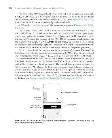
A 2D model is used to exemplify the optimization process (Morega et al., 2018),
Fig. 6.10.
The diameter of the blood vessel is d 5 6 mm. The bidimensional size of a 6-mm
3 2
thick PM of V 5 1.2 cm volume is, here, 0.2 cm . In the search for the optimal geo-
metric aspect ratio of the permanent magnet,A(A 5 height over width) that may provide
for best MDT effect, the volume of the PM, Vol, is constraint, which further sets
the total free PM energy, W m 5 Ð BUHÞ=2dvDVolU B rem UH c Þ=2(Fig. 6.10). It should
Vol ð ð
be mentioned that the resulting “optimum” elemental cell is rather a compromise between
the largest force, its orientation, and its area of action, rather than an optimum optimorum.
Fig. 6.11 (top) shows the optimization for the elemental cell (a single PM block) as
bell-shaped curves for the magnetic forces acting upon the MAF, F (streamwise) and
mg;x
F (orthogonal), where F 5 Ð Þ dxdy, S is the area of the MAF channel.
mg;y mg xjyÞ S f mg xjyð
ð
To compare these results with those in the following stages of optimization, SW (the
PM block width) is used in the abscissa instead of A. Both curves show off maxima,
with different values and locations though. The vertical force acts into attracting the
MD towards the PM, whereas the horizontal component may influence (enhance or
oppose) the flow. It can be inferred that the PM has to be placed so that the tumor is
located between the magnet and the blood vessel carrying the medication. Furthermore,
for pulsating flow conditions the action of F is more significant during the minima
mg;x
of the flow rate (Morega et al., 2018; S˘ andoiu, 2019; S˘ andoiu et al., 2019).

Symmetry
axis
Magnetic insulation

Permanent
magnet

Nonmagnetic
Magnetic fluid
(blood and MD)

y
x
Figure 6.10 The 2D model and the magnetic field boundary conditions. Symmetry is used to
reduce the computational domain.