Page 201 - Computational Modeling in Biomedical Engineering and Medical Physics

190 Computational Modeling in Biomedical Engineering and Medical Physics

Table 6.1 (S˘ andoiu, 2019) lists the optimization results NS 5 3, 4, and 5 identical
blocks. The GS limiting cases only are given here. SW, related to GS, is the running
the optimization parameter.
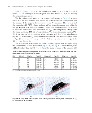
The three-dimensional results (see the magnetic field spectra in Fig. 6.14) are con-
sistent with the bidimensional ones, smaller but of the same order of magnitude, and
the maxima of the magnetic forces decrease when GS increases. The reason is that
the extrapolated 2D MAF volume is almost half the three-dimensional one, while the
average magnetic flux field tube is shorter. Hence, the bidimensional model is prone
to produce a more intense field. Moreover, is a F mg;x force component, orthogonal to
the stream and to the PM axis of magnetization. The three-dimensional maxima SW-
shift is less apparent but, interestingly, when compared with their bidimensional coun-
terparts, the maxima of F mg;y (attraction to the PM) occur later downstream than those
of F mg;z (stream-wise). The design with the highest magnetic forces corresponds to
GS 5 1mm(Fig. 6.15).
The MAF stationary flow under the influence of the magnetic field is analyzed using
the computational domain presented in Fig. 6.12B,and Fig. 6.14 shows the magnetic
field and the flow field for NS 5 1, 5. The wider spatial coverage of the magnetic field
Table 6.1 Magnetization forces maxima recorded along the top edge of the blood vessel and the
design parameters for different PM arrays.
NS ( ) GS (mm) SW opt (mm) F mg;x (N) SW opt (mm) F mg;y (N) SW opt (mm) F mg;z (N)
3 1 7.4 0.019051 8.6 0.272633 8 0.07751
6 7.6 0.012235 8.8 0.181689 8.4 0.038709
4 1 8.8 0.015457 10 0.262231 9.8 0.087083
6 8.8 0.011722 10 0.198195 9.2 0.04515
5 1 6.2 0.02113 7 0.2621 6.2 0.056329
6 6.4 0.011493 7.4 0.157431 6.8 0.020921
GS, Gap size; NS, number of slope; PM, permanent magnet.

Figure 6.14 Magnetic flux density (blue lines), velocity (red lines), and magnetic forces (arrows). (A)
NS 5 1 block. (B) NS 5 5 blocks.