Page 199 - Computational Modeling in Biomedical Engineering and Medical Physics

188 Computational Modeling in Biomedical Engineering and Medical Physics

The PM may be divided into NS 5 2, 3, etc. identical, equally spaced blocks, a
sequence which points out that for increasing NS and spacing, GS, in between them,
the magnetic blocks act more and more as independent PMs.
The second stage of optimization aims the first order constructal ensemble,NS 5 2. The
block width, SW (7 10 mm) and the spacing between them, GS (1 6 mm) are the opti-
mization parameters. The magnetic volume of each block is Vol. Fig. 6.11 (middle and bot-
tom) shows the results in the third stage of optimization when NS 5 3, the PMs of
volume Vol, for two limiting cases, GS 5 1mm and GS 5 6 mm. Quasi-independent,
noninteracting PMs may result for GS . 6 mm. The maxima of F and F decrease
mg;x mg;y
with GS by half (from 6 to 1 mm), for almost the same values of GS. It may be concluded
that GS 5 1 mm, the smallest GS, provides for an optimum. The optimal configuration
was found in the interval SW 5 3 4 mm. Depending on the morphology and the loca-
tion of the targeted tumor volume, the therapist may decide the optimal configuration for
the PM array.
The same analysis (GS and SW optimization) was performed for NS 5 4, 5, and
6blocks. Fig. 6.11 depicts F (middle) and F (bottom) for GS 5 1mm and
mg;x mg;y
GS5 6 mm, for NS5 3, 5. When comparing with NS 5 3, the maximum F for
mg;y
NS 5 5 occurs for a thinner (slender) block (SW 5 0.002 mm).
Although insightful, the bidimensional analysis may not account for the “duct” type of
flow of the MAF and for the third component (perpendicular to the plane) of the mag-
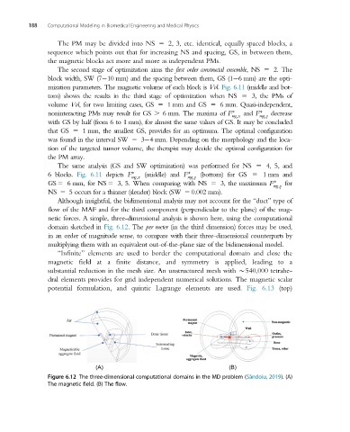
netic forces. A simple, three-dimensional analysisisshown here, using the computational
domain sketched in Fig. 6.12.The per meter (in the third dimension) forces may be used,
in an order of magnitude sense, to compare with their three-dimensional counterparts by
multiplying them with an equivalent out-of-the-plane size of the bidimensional model.
“Infinite” elements are used to border the computational domain and close the
magnetic field at a finite distance, and symmetry is applied, leading to a
substantial reduction in the mesh size. An unstructured mesh with B540,000 tetrahe-
dral elements provides for grid independent numerical solutions. The magnetic scalar
potential formulation, and quintic Lagrange elements are used. Fig. 6.13 (top)

Figure 6.12 The three-dimensional computational domains in the MD problem (S˘ andoiu, 2019). (A)
The magnetic field. (B) The flow.