Page 235 - Computational Modeling in Biomedical Engineering and Medical Physics

224 Computational Modeling in Biomedical Engineering and Medical Physics

applicators relative to the quality of the AF (Stuchly and Esselle, 1992; Morega, 1999;
Morega, 2000). The same model could be applied to transcutaneous energy transfer or
mild heating of implanted metallic devices for medical purposes.
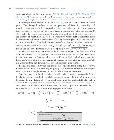
The computational domain is shown in Fig. 7.2, relative to a Cartesian coordinate
system. The biological medium is the homogeneous and isotropic conductive half-
space for z , 0, while z . 0 corresponds to the other half-space, of air; the magnetic
field applicator is represented here by a current-carrying coil with the contour Γ,
where iðtÞ is the variable current and dl is the elemental length of the cable, at a cer-
tain position of coordinates x 0 ; y 0 ; z 0 Þ. The induced electric field is computed inside
ð
the conductive half-space at the location Px; y; zÞ, for example along a nervous trunk,
ð
as is the case in PMS. The Euclidian measure of the distance between the elemental
p ffiffiffiffiffiffiffiffiffiffiffiffiffiffiffiffiffiffiffiffiffiffiffiffiffiffiffiffiffiffiffiffiffiffiffiffiffiffiffiffiffiffiffiffiffiffiffiffiffiffiffiffiffiffiffiffiffiffiffi
2
2
current, idl and point Px; y; zÞ is R 5 ð x2x 0 Þ 1 y2y 0 Þ 1 z2z 0 Þ , and its projec-
2
ð
ð
ð
p ffiffiffiffiffiffiffiffiffiffiffiffiffiffiffiffiffiffiffiffiffiffiffiffiffiffiffiffiffiffiffiffiffiffiffiffiffiffi
tion on the air tissue interface (xOy, z 5 0 plane) is ρ 5 ð x2x 0 Þ 1 y2y 0 Þ .
2
2
ð
Another assumption of the model is the quasisteady regime; the frequency of the
excitation current ð f , 10 kHzÞ and the average tissue conductivity (common values
for body tissues at low frequency electric stress, like σ 0:5S=m) lead to a penetration
depth much larger than the characteristic dimensions of anatomical domains, which in
turn are larger than the dimensions of the coils currently used in MS.
The relative balance between the sizes of the coils, the depth of the target for the
induced electric field, the operating frequency, the dielectric properties of biological
tissues support the simplified assumptions taken here into consideration.
First, the strength of the elemental electric field induced in the conductive half-space,
dE, due to the time-variable elemental electric current through the coil, idl, is expressed as
the sum of the contributions of two elemental components: the incident field, dE 1 ,and the
reaction field, dE 2 , each, in turn, formed by the contributions of a solenoidal component
and a potential component. At the process scale, the potential part of the incident field and
the solenoidal part of the reaction field are negligible, as shown by

@A 1 @A 2 @A 1
dE 5 dE 1 1 dE 2 5 d 2 2 gradV 1 1 d 2 2 gradV 2 Dd 2 2 gradV 2 ; ð7:5Þ
@t @t @t

(x ,y ,z )
0 0 0
idl
z y (Air)

x (Conductive tissue) R
(Long fiber) P(x,y,z)

Figure 7.2 The geometry of the computational model for the induced electric field (Morega, 2000).