Page 170 - Computational Retinal Image Analysis

3 Tools and techniques 165

Eliminating outliers
What constitutes an outlier in a data sample is a well-investigated topic in the literature,
which must be considered carefully in the light of one’s knowledge about the data at
hand. Much work exists on this topic in statistics and we refer the reader to Ref. [27]
for a comprehensive introduction. Well-known methods in computer vision are the
Least Median of Squares [28], RANSAC and its many variants [29, 30], and X84 [31].

Choosing an appropriate number of bins
Various rules compute the number of bins most likely, in some statistical sense,
to make the histogram of the sample at hand representative of the underlying dis-
tribution. Getting the number of bin wrong may make the histogram significantly
different from the underlying distribution (e.g., more bins than sample generates a
flat histogram). A commonly used rule is the one due to Freedman-Diaconis [32].
Briefly, given a sample of numerical measurements S = {s 1 , …, s N } not containing
outliers, the Freedman-Diaconis bin width, w, is
I RQ S ()
w = 2 ,
3 N
where IRQ(S) is the interquartile range of S and N is the total number of measurements.

2.00
Difference between OD and macula centered ZoneCVTORT
+1.96 SD
1.52
1.00

.00
Mean
-0.58
−1.00

−2.00

-2.68
−3.00 -1.96 SD

−11.00 −10.00 −9.00 −8.00 −7.00
Average of OD and macula centered ZoneCVTORT
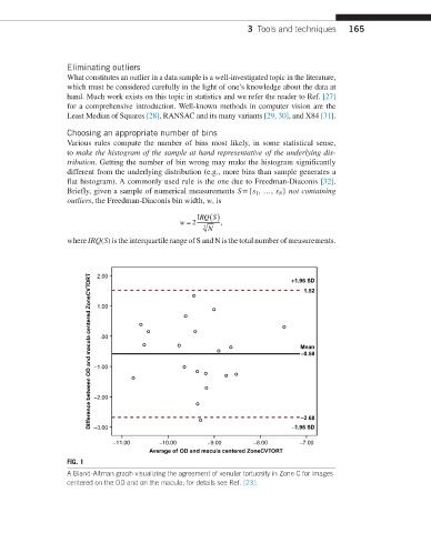
FIG. 1
A Bland-Altman graph visualizing the agreement of venular tortuosity in Zone C for images
centered on the OD and on the macula; for details see Ref. [23].