Page 117 - Computational Statistics Handbook with MATLAB

104 Computational Statistics Handbook with MATLAB

end
We can use this to generate a set of Poisson random variables with λ = 0.5 ,
and show a histogram of the data in Figure 4.10.

% Set the parameter for the Poisson.
lam = .5;
N = 500; % Sample size
x = cspoirnd(lam,N);
edges = 0:max(x);
f = histc(x,edges);
bar(edges,f/N,1,'w')
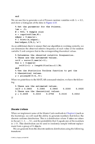
As an additional check to ensure that our algorithm is working correctly, we
can determine the observed relative frequency of each value of the random
variable X and compare that to the corresponding theoretical values.

% Determine the observed relative frequencies.
% These are the estimated values.
relf = zeros(1,max(x)+1);
for i = 0:max(x)
relf(i+1) = length(find(x==i))/N;
end
% Use the Statistics Toolbox function to get the
% theoretical values.
y = poisspdf(0:4,.5);
When we print these to the MATLAB command window, we have the follow-
ing

% These are the estimated values.
relf = 0.5860 0.3080 0.0840 0.0200 0.0020
% These are the theoretical values.
y = 0.6065 0.3033 0.0758 0.0126 0.0016

reet
ee
n
forfor
Dis DisDis Disc cr ccrr eett teeUUn iforform m
mm
UnUn
i
ii
When we implement some of the Monte Carlo methods in Chapter 6 (such as
the bootstrap), we will need the ability to generate numbers that follow the
discrete uniform distribution. This is a distribution where X takes on values
in the set 12 … N,,{ , } , and the probability that X equals any of the numbers
is 1 N⁄ . This distribution can be used to randomly sample without replace-
ment from a group of N objects.
We can generate from the discrete uniform distribution using the following
transform
© 2002 by Chapman & Hall/CRC