Page 258 - Computational Statistics Handbook with MATLAB

246 Computational Statistics Handbook with MATLAB

in the data set produce small changes in the value of the statistic. We illustrate
this situation in the next example.

Example 7.7
Researchers collected data on the weight gain of rats that were fed four dif-
ferent diets based on the amount of protein (high and low) and the source of
the protein (beef and cereal) [Snedecor and Cochran, 1967; Hand, et al., 1994].
We will use the data collected on the rats who were fed a low protein diet of
cereal. The sorted data are
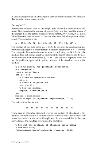
x = [58, 67, 74, 74, 80, 89, 95, 97, 98, 107];
ˆ
The median of this data set is q 0.5 = 84.5 . To see how the median changes
with small changes of x, we increment the fourth observation x = 74 by one.
ˆ
The change in the median is zero, because it is still at q 0.5 = 84.5 . In fact, the
median does not change until we increment the fourth observation by 7, at
ˆ
which time the median becomes q 0.5 = 85 . Let’s see what happens when we
use the jackknife approach to get an estimate of the standard error in the
median.

% Set up memory for jackknife replicates.
n = length(x);
reps = zeros(1,n);
for i = 1:n
% Store as temporary vector.
xt = x;
% Leave i-th point out.
xt(i) = [];
% Get the median.
reps(i) = median(xt);
end
mureps = mean(reps);
sehat = sqrt((n-1)/n*sum((reps-mureps).^2));
The jackknife replicates are:
89 89 89 89 89 81 81 81 81 81.

ˆ
(
ˆ
These give an estimated standard error of the median of SE Jack q 0.5 ) = 12 .
Because the median is not a smooth statistic, we have only a few distinct val-
ues of the statistic in the jackknife replicates. To understand this further, we
now estimate the standard error using the bootstrap.
% Now get the estimate of standard error using
% the bootstrap.
[bhat,seboot,bvals]=csboot(x','median',500);

© 2002 by Chapman & Hall/CRC