Page 256 - Computational Statistics Handbook with MATLAB

244 Computational Statistics Handbook with MATLAB

14 14
12 12
10 10
8 8
6 6
4 4
5 10 15 20 5 10 15 20
14 14
12 12
10 10
8 8
6 6
4 4
5 10 15 20 5 10 15 20

FI F U URE G 7. RE 7. 3 3
IG
GU
F F II GU RE RE 7. 7. 3
3
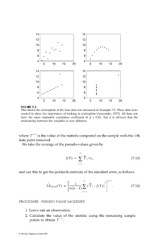
This shows the scatterplots of the four data sets discussed in Example 7.5. These data were
created to show the importance of looking at scatterplots [Anscombe, 1973]. All data sets
have the same estimated correlation coefficient of ρ ˆ = 0.82 , but it is obvious that the
relationship between the variables is very different.
i – ()
where T is the value of the statistic computed on the sample with the i-th
data point removed.
We take the average of the pseudo-values given by

n
)
⁄
JT() = ∑ T i n , (7.13)
i = 1
and use this to get the jackknife estimate of the standard error, as follows

⁄
n 12
ˆ 1 ) 2
SE JackP T() = -------------------- ∑ ( T i – JT()) . (7.14)
(
nn – 1)
i = 1
PROCEDURE - PSEUDO-VALUE JACKKNIFE

1. Leave out an observation.
2. Calculate the value of the statistic using the remaining sample
points to obtain T i – () .

© 2002 by Chapman & Hall/CRC