Page 251 - Computational Statistics Handbook with MATLAB

Chapter 7: Data Partitioning 239

% Fit a quadratic to the data.
[p2,s] = polyfit(xtrain,ytrain,2);
% Fit a cubic to the data
[p3,s] = polyfit(xtrain,ytrain,3);
% Get the errors
r1(i) = (ytest - polyval(p1,xtest)).^2;
r2(i) = (ytest - polyval(p2,xtest)).^2;
r3(i) = (ytest - polyval(p3,xtest)).^2;
end
We obtain the estimated prediction error of both models as follows,

% Get the prediction error for each one.
pe1 = mean(r1);
pe2 = mean(r2);
pe3 = mean(r3);
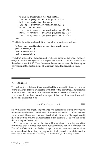
From this, we see that the estimated prediction error for the linear model is
0.86; the corresponding error for the quadratic model is 0.88; and the error for
the cubic model is 0.95. Thus, between these three models, the first-degree
polynomial is the best in terms of minimum expected prediction error.

7.3 Jackknife
The jackknife is a data partitioning method like cross-validation, but the goal
of the jackknife is more in keeping with that of the bootstrap. The jackknife
method is used to estimate the bias and the standard error of statistics.
Let’s say that we have a random sample of size n, and we denote our esti-
θ
mator of a parameter as

ˆ
,
,
(
,
θ = T = t x 1 x 2 … x n . ) (7.8)
ˆ
θ
So, might be the mean, the variance, the correlation coefficient or some
T
other statistic of interest. Recall from Chapters 3 and 6 that is also a random
variable, and it has some error associated with it. We would like to get an esti-
mate of the bias and the standard error of the estimate T, so we can assess
the accuracy of the results.
When we cannot determine the bias and the standard error using analytical
techniques, then methods such as the bootstrap or the jackknife may be used.
The jackknife is similar to the bootstrap in that no parametric assumptions
are made about the underlying population that generated the data, and the
variation in the estimate is investigated by looking at the sample data.

© 2002 by Chapman & Hall/CRC